Lesson 21: Transformers

Transformers

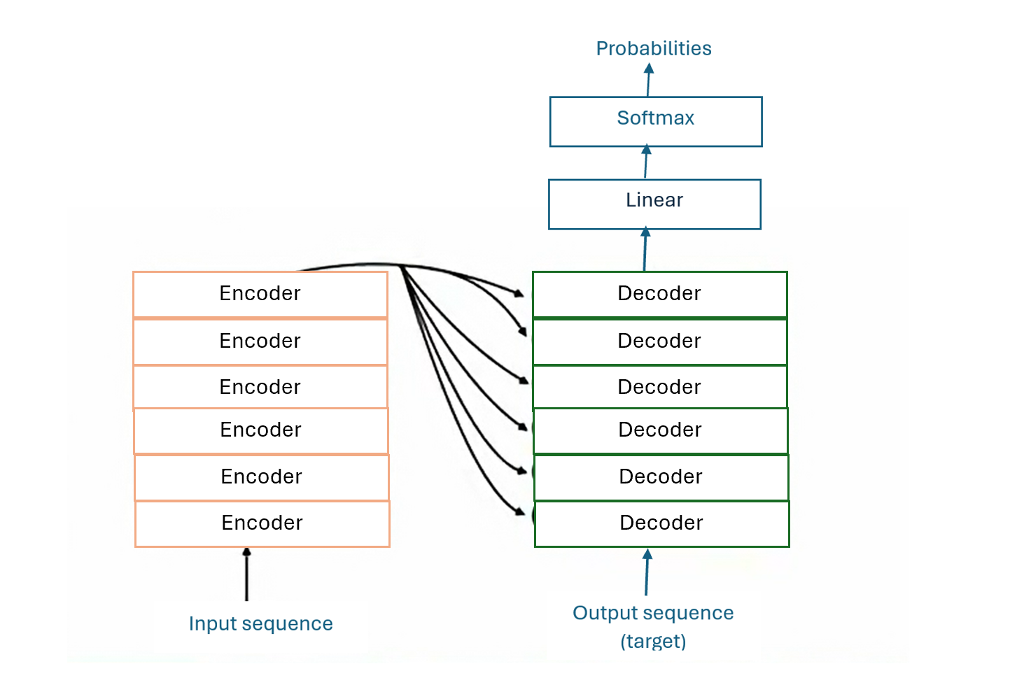
Transformers are the state-of-the-art architecture behind large language models and modern generative AI. Transformers neural network consisting of a stack of encoders and decoders leveraging self-attention mechanism. In the paper that introduced Transformers, Attention Is All You Need, six identical encoder blocks and six identical decoder blocks were used in the transformer architecture.

The figure below illustrates how a stack of encoder blocks and decoder blocks constitute a transformer.

Transformers are an improvement to RNN-based models. RNN models capture information using hidden states, and the hidden states in later time steps tend to forget information in earlier time steps. RNNS also process information sequentially in a recurrent manner, which could result to slow computation.

Transformers solve RNNs’ long memory and slow computation issues by capturing relevant information in a sequence using self-attention and processes sequence tokens in parallel respectively. Transformers have the following characteristics:

• use self-attention
• eliminate the need for recurrence
• process tokens in parallel
• faster to train

Transformer Architecture

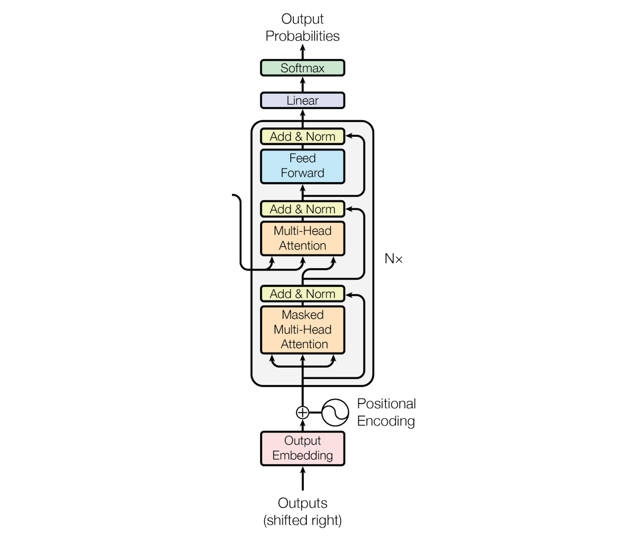
The Transformer architecture was first published by Vaswani et al. in 2017 in the paper, Attention Is All You Need. This was the paper that introduced the Transformer architecture as shown in the figure below.

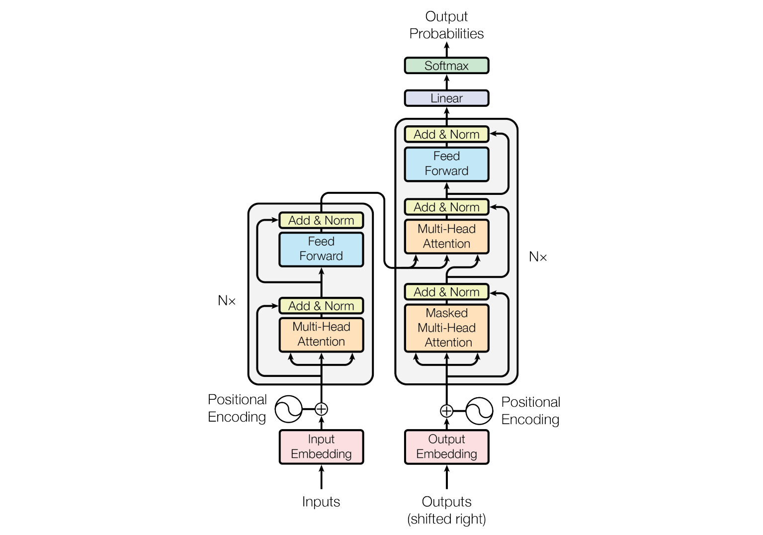
The transformer architecture has two main components, an encoder and a decoder.

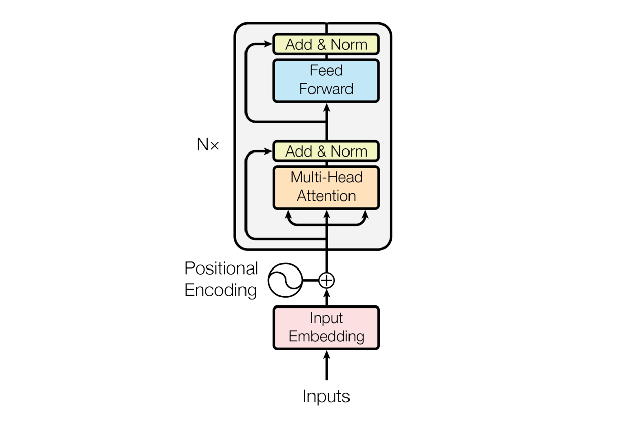
The Encoder

The encoder consists of a stack of \(N\) identical blocks. Each encoder block has a multi-head attention layer and a simple feed forward neural network.

Token Embeddings

The tokens in the input sequence are first converted into token embeddings (input embeddings). Pretrained embeddings are typically used though the embeddings could be trained from scratch. The embedding dimension of 512 is typically used as in the Attention Is All You Need paper. However note that an embedding dimension is a hyperparemeter that can be tuned.

Position encoding

Position encodings are computed and added to the input embeddings to obtain the final input embeddings (encoder’s input) that capture information about the meaning and positions of the tokens. A position embedding is a vector containing information about the position of a token.

• Each token (or token embedding) has a corresponding position encoding vector. Hence, the size of a position encoding vector is the same as the size of an input embedding vector (512).
• Position embeddings can be computed in various ways but sine and cosine position encodings were used in the Attention Is All You Need paper.

A positional embedding for a token is computed using the position of the token in the sequence and the indexes of the elements in the embedding vector as follows:

\[\begin{align} \text{PE}(\text{pos}, 2i) &= \sin\left(\frac{\text{pos}}{10000^{2i / d_{\text{model}}}}\right) \\ \text{PE}(\text{pos}, 2i+1) &= \cos\left(\frac{\text{pos}}{10000^{2i / d_{\text{model}}}}\right) \end{align}\]

where:

• \(\text{pos}\) is the position of the token in the sequence.
• \(i\) is the dimension index within the embedding vector (\(i=0, 1, 2, ..., 512\)).
• \(d_{\text{model}}\) is the dimensionality of the model (size of the embedding vector). Note that the size of the input and output embedding vectors are consistent through out the encoder and decoder networks of the Transformer.

The positional encoding vector of the first token takes the form: [PE(0, 0), PE(0, 1), PE(0, 2), PE(0, 3), …, PE(0, 512)]

The positional encoding vector of the second token takes the form: [PE(1, 0), PE(1, 1), PE(1, 2), PE(1, 3), …, PE(1, 512)], and so on.

The positional encoding function computes positional encodings up to a given maximum sequence length (max_len) and dimension (d_model). For fixed-length sequences in transformers, positional encoding is computed once and reused for every sentence.

Multi-head attention

The attention mechanism generates attended representations of tokens from the input embeddings. An attended representation is an embedding that captures relevant contextual information for a token in the sequence.

A multi-head attention is basically a set of single self attention layers implemented in parallel or simultaneously. So, to understand multi-head attention, we need to understand self attention. A self attention layer is called a head and a collection of self attention layers implemented in parallel is called multi-head attention layer.

The self-attention layer uses three weight matrices called Query (\(W_Q\)), Key (\(W_K\)) and Value (\(W_V\)) weight matrices to transform the input embeddings into query (\(q\)), key (\(k\)), and value (\(v\)) vectors as shown below.

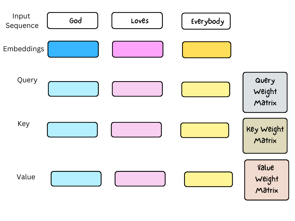
In practice, instead of multiplying the input embedding vectors separately by the weight matrices \(W_Q\), \(W_K\), and \(W_V\), the embedding vectors are packed into a matrix \(X\) with dimensions \(d_{seq}\) x \(d_e\), where each row of \(X\) is an embedding vector.

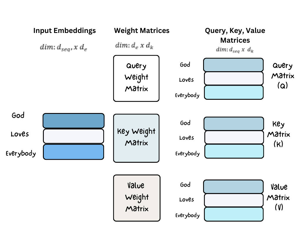
Multiplying \(X\) by \(W_Q\), \(W_K\), and \(W_V\) gives \(Q\), \(K\), and \(V\) respectively. The \(ith\) rows of \(Q\), \(K\), and \(V\) matrices contains the \(ith\) query (\(q\)), key (\(k\)), and value (\(v\)) vectors respectively. \(q\), \(k\), and \(v\) have the same dimension \(d_k = d_k = d_v\).

• \(d_{seq}\) is the sequence length. For large language models, the sequence length could be \(N\) = \(d_{seq}\) = 1024, 2048, or 4096 tokens.
• \(d_e\) is the size of the input embedding (for example, 512).
• \(d_k\) is dimension of the key vector (for example, 64). 64 is used so that with 8 attention heads, we can concatenate the attention vectors to a vector of 512 for each token with the original embedding dimensionality.

The figure below shows how to transform input embeddings into query, key, and value matrices through matrix multiplication with weight matrices.

The query (Q), key (K), and value (V) matrices obtained from the above transformation can then be used to compute self-attention as a scaled dot-product attention as follows:

1. Compute Attention Scores: \(\text{Attention Scores} = \frac{Q \cdot K^T}{\sqrt{d_k}}\)

   The attention scores computed are stored as a matrix where the \(ith\) row contains the attention scores for the \(ith\) token, indicating the similarity between \(ith\) token and each token in the sequence. The elements of the \(ith\) row (\(a_{ij}\)) represents how much the \(ith\) token attends to each \(jth\) token or how much each \(jth\) token is contextually relevant to the \(ith\) token. A higher \(a_{ij}\) means the \(ith\) token places more importance or attention on the j-th token. The dimension of the attention score matrix is \(d_{seq}\) x \(d_{seq}\).

2. Apply Softmax: \(\text{Attention Weights} = \text{softmax}\left(\frac{QK^T}{\sqrt{d_k}}\right)\)

   Softmax is applied along each row to obtain the attention weights for each query, to scale attention scores into attention weights, ensuring the attention scores for each token sum to 1.

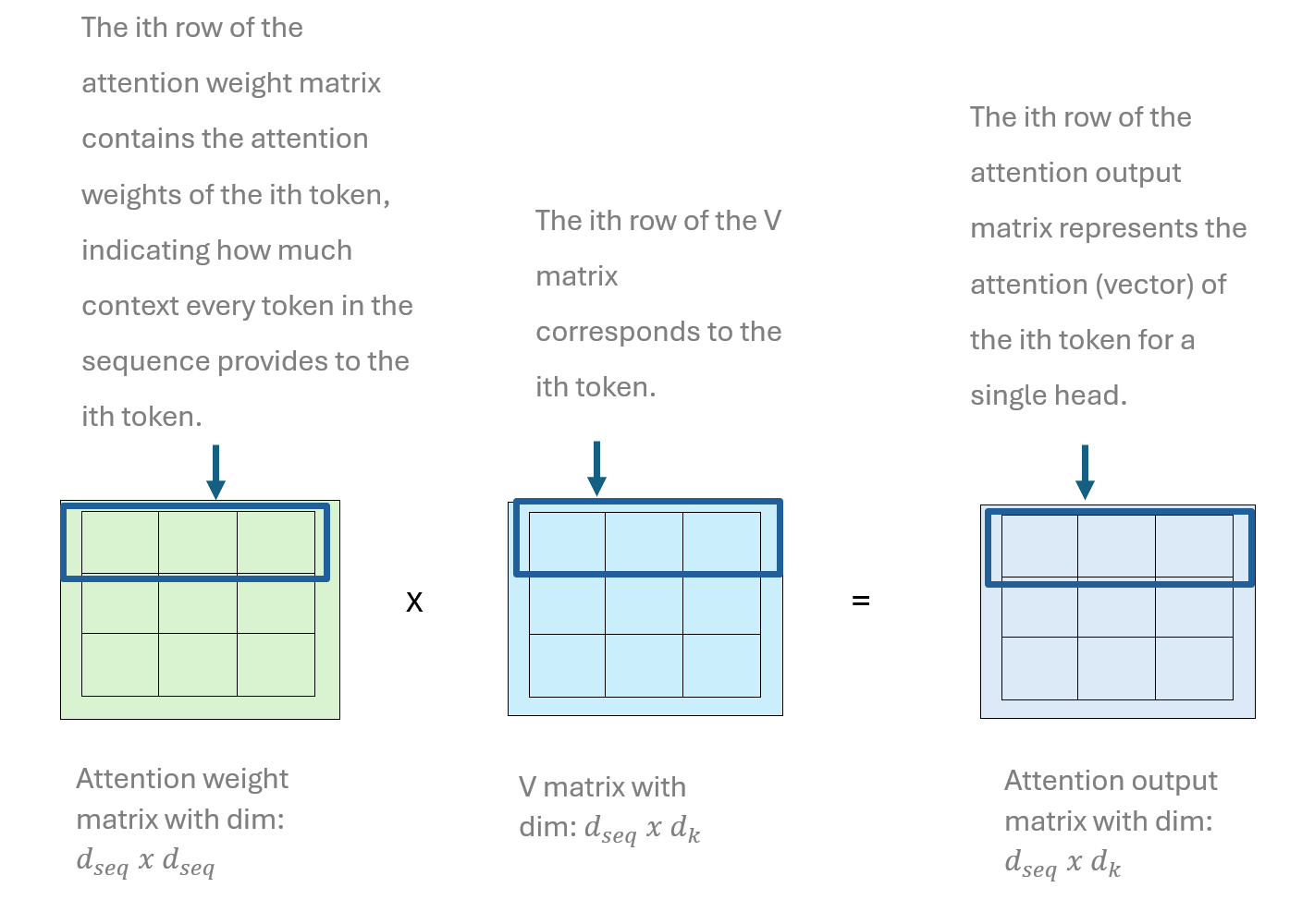
3. Compute Weighted Sum: \(\text{SelfAttention}(Q, K, V) = \text{softmax}\left(\frac{QK^T}{\sqrt{d_k}}\right) V\)

   Each row of the self attention output matrix is the weighted sum of values, where the weights are the softmax of the attention scores. The matrix multiplication that produces each attention output vector in the attention output matrix is the same as applying each weights in the attention vector to its corresponding value vector, then computing an element-wise sum of the weighted value vectors.

Self-attention is a fundamental operation in transformers that enables each token in a sequence to selectively capture contextual information from other tokens within the same sequence. Self-attention involves updating each token embedding to selectively capture contextual information for the token.

Self-attention is implemented through a self-attention layer, one of the core layers of a transformer block. The self-attention layer updates the embeddings of each token in the input sequence through the application of weights.

The vectors or attention representations resulting from the self attention mechanism capture the meaning, positions and contextual information of tokens.

The transformation of input embeddings into attention representations as illustrated above is achieved through a single-head attention. The implementation of several single-head attentions in parallel is called multi-head attention.

Each attention head computes attention weights independently, allowing for parallel computation of attention scores. The attention output matrices of the multi-head attention are concatenated to obtain the final attention matrix output for the input sequence.

The number of attention heads in a multi-head attention is given as:

\[ h = \frac{d_{model}}{d_k} \] Based on this formula above, when the attention outputs in multi-head attention are concatenated, the dimension of the final attention matrix should be \(d_{seq}\) x \(d_{model}\)

In the original transformer paper:

• \(d_{model} = d_e = 512\)
• \(d_k = d_v = 64\)
• \(h = 8\)

Self attention can be visualized to show the extent to which each word in the sequence attends to a particular word. For example, in the “Attention Is All You Need” paper, the token, The provides more context to the token, Law which in turn provides context to the token, its as shown below.

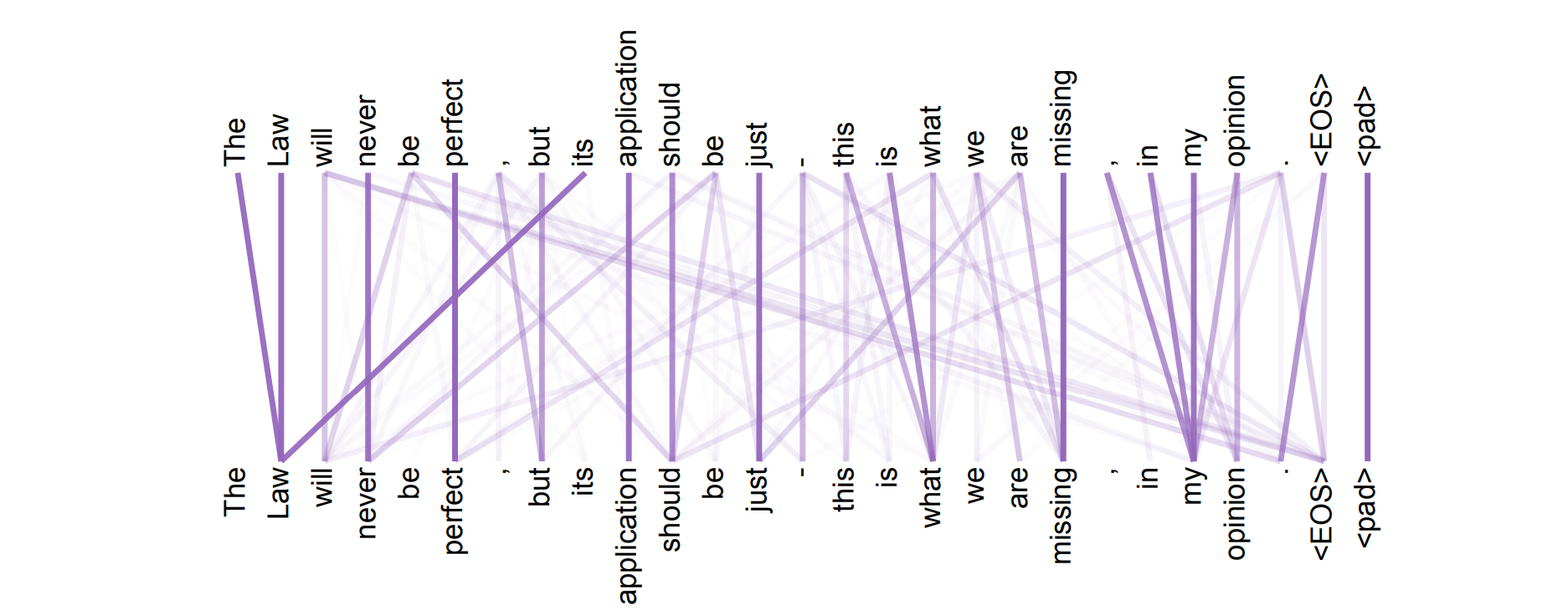When a word attends to other words, it means that the word gathers contextual information from other words. For example, the attention mechanism allows the word “Law” to attend to “The”, “Law” and “its”.

Add & Norm Layer

Within each encoder block, some operations are applied to the output of the sub-layer (multi-head attention layer and feed forward network) using the Add & Norm layer (layer normalization).

The Add operation of the Add & Norm Layer of adds the input of the sub-layer to the output of the sub-layer to ease the flow of gradient during backpropagation. This addition process is known as residual connection: \(x + \text{SubLayer}(x)\).

The Norm layer computes the mean and standard deviation of each vector (resulting from the Add operation) and uses these statistics to convert the entries of each vector into standard or z-scores: \(\text{LayerNorm}(x + \text{SubLayer}(x))\).

The purpose of the Add & Norm layer obtain output that would prevent gradient from diminishing during backprorogation as well as stabilize the distribution of outputs across layers by scaling, to improve the model performance.

Feed forward neural network

The output of the Add & Norm layer is a sequence of vectors associated with the tokens in the input sequence. These vectors are fed into a fully connected simple feed forward network independently, hence the processing of the vectors could be parallelized across multiple GPUs. The FFNN consists of two a hidden layer and and an output layer.

The hidden layer processes each input vector \(\mathbf{x}_i\) associated to the \(ith\) token in the input sequence as follows:

\[ \mathbf{h}_i = \mathrm{ReLU}(\mathbf{x}_i \mathbf{W}_1 + \mathbf{b}_1) \]

The output layer processes each output vector of the hidden layer \(\mathbf{h}_i\) as follows:

\[ \mathbf{y}_i = \mathbf{h}_i \mathbf{W}_2 + \mathbf{b}_2 \]

Each output vector \(\mathbf{y}_i\) of the feed forward network corresponding to the \(ith\) token is further processed through the Add & Norm layer.

The output of one encoder block serves as input embeddings into the subsequent encoder or transformer block. Each encoder block applies the same series of operations to the input embeddings. The final output of the encoder stack is a sequence of vectors, where each vector captures the meaning, position and context of each token in the input sequence.

The Decoder

Similar to an encoder, a decoder consists of a stack of \(N\) identical decoder blocks. Each decoder block has a masked multi-head attention layer, a multi-head attention and a simple feed forward neural network.

The decoder works in a similar way as the encoder. During the training of a transformer model for machine translation or any sequence-to-sequence task, the training sample consists of an input sequence (for example: God Loves Eerybody) in the source language (such as English) and an output sequence (for example: <SOS> Dieu aime tout le monde) in the target language (French).

The input embeddings are passed into the encoder to generate embeddings that capture the meaning, positions and context of the tokens in the input sequence. The output of the encoder stack is used to create a value and key matrices for the multi-head attention layer of the decoder.

Enriching input embeddings with positional embeddings

The output sequence (<SOS> Dieu aime tout le monde) in the target language is passed as input into the decoder. The output sequence is first converted into output embeddings. The embeddings are then augmented with positional embeddings.

Masked multi-head attention

The enriched output embeddings are then passed into a masked multi-head attention layer. Masked attention ensures that the current token can only attend to itself or previous tokens. That means, only previous tokens or the current token itself can provide context to the current token.

Masking prevents the model from looking ahead into future tokens when making prediction during training. That is, masking forces the model to learn to predict each token in the output sequence based only on the tokens that precede it, as would be the case during inference. Without masking, the decoder could cheat during training by using information for future tokens to make predictions.

Add & Norm layer

The Add & Norm layer is then applied to the input and output of the masked multi-head attention layer to obtained embeddings that improve the training speed.

Multi-head attention layer

The output embeddings of the decoder’s Add & Norm layer are stacked into a matrix \(Y\), fed into the multi-head attention layer, and projected into query vectors, stacked in a matrix \(Q\). The encoder’s output \(E\) is also passed into the multi-head attention layer and projected into keys (\(K\)) and values (\(V\)).

For each token:

• \(Q = W_Q \cdot Y\)
• \(K = W_K \cdot E\)
• \(V = W_V \cdot E\)

The multi-head attention in the decoder is called cross-attention (or encoder-decoder attention). Cross-attention mechanism allows each token in the output sequence (decoder’s input) to attend to all tokens in the input sequence (encoder’s output). Specifically, the \(ith\) token in the query sequence attends to every \(jth\) token in the key-value sequence. This enables the decoder to incorporate relevant information from the entire input sequence.

The output of the multi-head attention layer is further processed through another Add & Norm layer. The output of the Add & Norm layer consists of a sequence of vectors.

Feed forward neural network

The embedding vectors obtained from the Add & Norm layer are then processed through a feed-forward neural network to produce another sequence of vectors. A final Add & Norm layer is applied to the output of the feed forward network to obtain the output of the decoder block. The output of the decoder block is further process by subsequent decoder blocks until the final output (hidden state) \(H\) of the decoder stack is obtained.

The linear layer

The linear layer transforms the output (hidden state) of the decoder stack through a linear transformation into logits. The hidden state \(H\) of decoder stack consists of sequence of vectors stacked together into a matrix, where the vector in the \(ith\) row corresponds to the \(ith\) token.

The linear layer allows the model to project the decoder’s output into the vocabulary space.

The linear transformation in the linear layer is as follows:

\[ L = H \cdot W_0 + b_0 \] where:

• \(𝐻\) represents the decoder’s output or hidden states, with dimensions \(m\) x \(d_{model}\). Note that \(m\) is output sequence length and \(d_{model}\), the embedding size through out the encoder and decoder layers.
• \(W_0\) is the weight matrix in the linear layer with dimensions \(d_{model}\) x \(|v|\) and \(b_0\) is the bias term.
• The output \(L\) is a matrix of logits with dimensions 𝑚 x 𝑉. The \(ith\) row of matrix L corresponds to the logits of the \(ith\) token in the sequence, and the \(jth\) column corresponds to the score of the \(jth\) word in the vocabulary.

The softmax layer

The Softmax layer is used to convert the logits into probability distributions. The softmax function is applied to each row of matrix \(𝐿\) to produce a matrix of probabilities \(P\).

\[ 𝑃= \text{Softmax}(𝐿) \] The \(ith\) row of matrix \(P\) represents the probability distribution over the vocabulary for predicting the next token in the sequence, given the context up to and including the \(ith\) token in the output sequence.

Training the Transformer Model

For a machine translation task, each training pair (input sequence, output sequence) is fed into the transformer model (encoder and decoder) to generate the softmax probability distributions over vocabulary during a single forward pass.

Teacher forcing is implemented during training, where the decoder uses the true token \(y_{t-1}\) (instead of a generated token) from the shifted sequence at time step t to predicts the next token \(y_t\). Teacher forcing is implemented by shifting the output sequence to the right by one position: appending \(<SOS>\) at the beginning of the output sequence.

After computing the probability distributions over the vocabulary for each time step, the loss for each time step is computed. The model training objective or loss is to maximizing the probability of the actual next word given the input context.

The cross-entropy loss at each time step is computed as:

\[ l_t = -\log{\hat{y}_{t, target}} \] where \(\hat{y}_{t, target}\) is the probability of generating the actual next word at time step t.

The total loss \(L\) is calculated as follows:

\[ L = \frac{1}{m} \sum_{t=1}^{m} l_t \]

where:

• \(m\) is the length of the output sequence.
• \(l_t\) is the cross-entropy loss at time step t.

Once the total loss is computed, backpropagation is used to calculate the gradients of this loss with respect to each of the model’s parameters. The calculated gradients are then used by an optimization algorithm (e.g., Adam) to update the model parameters in the direction that reduces the total loss.

Inference with the Transformer Model

During inference, the decoder processes the initial output sequence \(<SOS>\) (decoder’s input) and output of the encoder and computes a probability distribution over the vocabulary. The next token is then sampled or generated from the probability distribution. The generated (or predicted) token is appended to the output sequence and the new sequence is used as the decoder’s input.

The updated decoder’s input sequence is processed through the decoder to generate the next token. That is, the decoder input is enriched with positional encodings and passed through the masked multi-head attention layer to capture the contextual information for each token in the output sequence. The Add & Norm layer is applied to the output of the masked multi-head attention layer.

The cross-attention layer uses the representation for the current position produced by the previous layer to create a query, and the encoder’s output representations to create the keys and values. The cross-attention (multi-head attention) layer then produces another representation for the current token that captures contextual information from the encoder. This representation for the current token is then processed through the rest of the decoder layers to generate the next token.

The next token is used to update the decoder’s input sequence and the process is repeated until the predicted token \(<EOS>\) is generated. The decoder in a transformer model typically operates in an autoregressive manner during inference where the model generates a sequence of tokens, one token at a time, conditioned on previously generated tokens.

Note that the decoder uses a sampling strategy such as greedy sampling to generate a token. Greedy sampling selects the token with the highest softmax probability. The generation of a token conditioned on some context text or prompt is called conditional generation. The maximum input sequence length for transformers is typically 1024, 2048 or 4096. The context length for transformers is the same as the sequence length since the attention mechanism allows each word to attend to every word in the input sequence.