Lesson 15: Language Models
Language Models
Language models or probabilistic language models are the models that power systems such as auto-correction and auto-completion systems. Search engines use large language models for spelling correction, sentence completion or web search suggestions.
Language models are used to predict the next word or sequence of words in a sentence. Probabilistic language models estimate the probability of a sentence or a word given a sequence of previous words.
Probabilistic language modeling involves the assignment of probability. For example:
A speech recognition system compares the probability of sentences that sound in a similar way and outputs the sentence with the highest probability: \(P(\text{I saw a van}) > P(\text{eyes awe Evan})\)
An auto-suggestion system finds the next word or token with the highest probability given the context words: \(P(\text{Year|Happy New})\) may have the highest probability compared to the probability of other words in the training corpus given the context, “Happy New”.
Estimating Probabilities in Language Modeling
Probability of a Sequence of words
The chain rule allows us to compute the joined probability of a sequence of words.
The formula above shows that the probability of a sequence of words is the product of the probability of each word given the previous words (or history).
Word Probability
A simple approach for computing word probability is to use word frequency or count as follows.
Probability of a Word Given Previous Words
The rule of conditional probability is used to calculate the probability of a word given previous words.
If we want to predict the next word in the sentence, My duaghter likes ___, we could find the probability distribution over the next word given the previous words in the sequence by counting how many times the previous words and next word occur together and how many times the previous occur in the training corpus.
\[\begin{align} P\text{(oranges |My daughter likes to eat)} = \frac{\text{C(My daughter likes to eat oranges)}}{C(\text{My daughter likes to eat})} \end{align}\]
Challenges with Count Approach to Probabilistic Language Modeling
The problem with finding the probability of a sequence of words \(P(w_{1:t})\) is that there would be too many computations to make as shown from the chain rule. The chain rule involves computing several conditional probabilities.
Additionally, the challenge with finding the probability distribution of the next word given the previous words in sequence is that the corpus may have one or a few specific examples of previous words and next word together. This can result to a sparsity issue and unreliable estimates of probability. The estimate may be unreliable because they may not accurately reflect the true likelihood of encountering that sequence in the future.
A better way to estimate these probabilities is to use n-grams where only a few sequence of previous words are used to estimate the probability of the next word instead of the entire history of the next word.
N-gram Language Models
N-gram language models use \(n\) sequence of words (or n-grams) to estimate probability. For example, uni-gram, bi-gram and tri-gram language models can be written as follows:
Unigram language model: The unigram language model uses only one token or word. This model does not account for any context words, hence it is technically a bag of words model. \[P(w_t) = \frac{C(w_t)}{T}\] Bigram language model: The bigram model uses two nearby tokens or words. This model computes the probability of a word given the previous word. \[P(w_t|w_{t-1}) = \frac{C(w_{t-1}, w_t)}{C(w_{t-1})}\]
Trigram language model: The trigram model uses three consecutive sequence of tokens or words. This model computes the probability of a word given the preceding two word.
\[P(w_t|w_{t-2}, w_{t-1}) = \frac{C(w_{t-2}, w_{t-1}, w_t)}{C(w_{t-2}, w_{t-1})}\] N-gram language modeling approximates the probability of a word given it’s entire history using only the last few preceding words instead of the entire history of words.
All n-gram models are Markov models because n-gram models use the Markov assumption that the probability of a word depends only on a fewer previous words rather than the entire history of words in a sequence. Markov models are the class of probabilistic models that assume we can predict the probability of some future unit without looking too far into the past.
Note that, log probabilities, \(\log{P(w_{1:t})}\) are usually computed instead of probabilities, \(P(w_{1:t})\) because log probabilities requires adding conditional probabilities which give reasonable numbers that are easily stores.
Computing the probability of a sequence of words requires the multiplication of conditional probabilities which can lead to numerical underflow or very small numbers that are difficult to store.
Bigram Conditional Probabilities
The table below shows bigram probabilities for eight words in the Berkeley Restaurant Project corpus of 9332 sentences (Jurafsky & Martin, 2024).
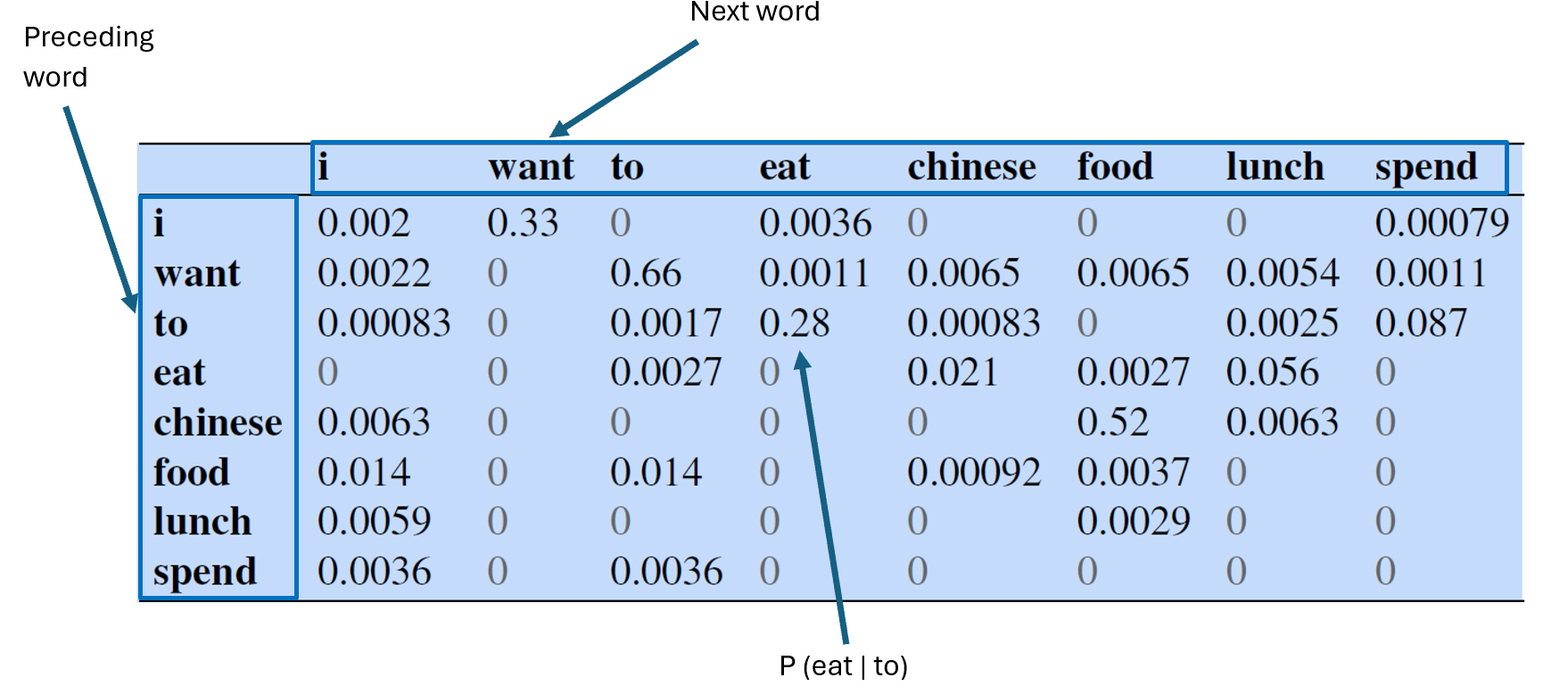
The bigram conditional probabilities on this table are obtained as follows:
- The bigram counts (counts of each word and its preceding word occurring together) are first computed as shown below:
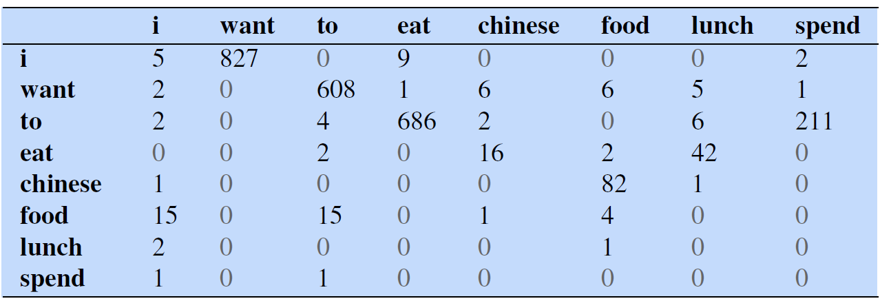
- Then the bigram counts in each cell are then normalized by dividing each cell by the counts of the appropriate unigram in its rows. The counts of unigrams in the rows are as shown below:

From the bigram conditional probability matrix (or table), the probability of sentences or a sequence of word can be approximated. For example:
\[\begin{align} P(\text{i want food}) &= P(I|<s>)P(want|i)P(food|want)P(</s>|food) \\ &= 0.25*0.33*0.0065*0.68 \\ &= 0.00036465 \end{align}\]
A speech recognition system can compute the probability of several sentences that sound in a similar way, then outputs the one that has a higher probability. For example, \(P(\text{i want to eat})\) can be compared with \(P(\text{i one two eat})\), then the sentence with the highest probability will be displayed. The conditional probabilities used to compute the probabilities of sentences are obtained from the probability matrix generated from the training corpus.
Also, the conditional probability matrix can be used to predict next words in new sentences. For example, based on the bigram conditional probabilities in the matrix above, what do you think would be the next word in this sentence, i need to ___? Given the preceding word, to, the next word with the highest probability is eat, so we can predict eat as the next word.
Though we have illustrated how to use bigram language models for estimating conditional probabilities of words and probabilities of sequences of words, in practice, trigram, 4-gram and even 5-gram are used in a similar way when there is sufficient data.
Also note that for larger n-grams, we can assume more context at the beginning and end of a sentence using more \(<s>\) or \(</s>\) respectively when computing conditional probability. For example, for a trigram, we could compute the probability \(P(i|<s><s>\) at the beginning of a sentence.
Evaluating Language Models
Extrinsic and Intrinsic Evaluation
N-gram language models can be evaluated using extrinsic and intrinsic approaches. For an extrinsic approach, two or more language models are used in a real nlp task such as speech recognition and their performances are computed and compared.
For example, two models such as bi-gram and tri-gram language models are embedded in a speech recognition system and used to convert speech to text. The proportion of words transcribed correctly by each model is then computed as the accuracy of the model. The accuracy for the bigram and trigram model are then compared.
Extrinsic evaluation can be expensive because the nlp pipeline needs to be run multiple times to get the accuracy of each model being evaluated. An extrinsic evaluation is also time consuming and may not generalize well to other applications. A model’s accuracy may not be the same for a speech recognition task and a machine translation task when extrinsic evaluation is used. For these reasons, intrinsic evaluation of language models is preferred.
An intrinsic evaluation uses an intrinsic metric to evaluate the performance of the model independent of the application. That means, with intrinsic evaluation, there is no need to embedded the model into the application. An intrinsic metric such as perplexity can be used for intrinsic evaluation.
Training and Test Sets
A training set is used to train the model. That is, a training set is the data used to learn the parameters of a the model. For a language model, the n-gram counts can be viewed as the parameters of the model.
A test set is used to evaluate the performance of the model. Evaluating a model with a test set allows us to understand how well the model generalizes to unseen or new data. The test set should have the following characteristics:
- The test set is a dataset that the model has not seen.
- The test set should be representative of the data, which means the test set should look like the training set.
Note that generic and specific language models can be trained. Generic language models should be trained with generic data or data from across different domains and sources. Specific language models should be trained and tested with domain specific data. For example, medical or legal language model can be trained.
Perplexity
Perplexity is founded on the idea that, a good language model assigns high probability to the next word that actually occurs or generally assigns a higher probability to the entire test set. So, when comparing two n-gram language models, the better models assigns a higher probability to the test set.
The perplexity, \(PP(w_1, w_2, w_3, ... w_{t-1}, w_T)\) on a test set is the inverse of the probability of the test set normalized by the length of the text.
The longer the text, the smaller it’s probability, the per-word perplexity (or simply, perplexity) is normalizes the inverse of the probability of the text using the length of the text, T, by applying the T-th rooth to the inverse probability of the text.
Challenges with N-gram Language Models
Storage Problem
Storage is needed to store all n-grams in the corpus. When the size of the corpus or “n” increases, more storage is needed to store more n-grams. Storing all these n-grams and their associated counts or probabilities requires more memory.
Sparsity Problem
N gram works well if the test set looks like the training set. If there is a word in the test set that is not in the training set, this will lead to:
- zero n-gram counts.
- zero conditional probability of the word.
- zero probability of the test set if the probability of any word in the test set is 0.
- undefined perplexity as 1 divided by a zero probability is undefined.
Sparsity problems are worse when “n” in the n-gram is large, making it difficult to find instances where context and next words occurred together in the training corpus, resulting to n-gram counts and zero probabilities.
Solution to the Sparcity Problem
Smoothing
One common approach to solving the zero n-gram probability problem is to use Laplace smoothing. Laplace (add 1) smoothing involves adding 1 to the n-gram counts before normalizing the counts into conditional probability. The probability of a word with Laplace smoothing is computed as: \[ P_{add-1}(w_t) = \frac{C(w_t)+ 1}{T + V} \] where \(T\) = text size and V = vocabulary size. V is added to the vocabulary because every unique word has been counted one more time.
The bigram conditional probability of a word with Laplace smoothing is computed as:
\[ P_{add-1}(w_t|w_{t-1}) = \frac{C(w_{t-1}, w_t) +1}{C(w_{t-1})+V} \]
Back-off
Back-off is a technique used only when higher-order n-gram count is zero. For example, if we were estimating a trigram probability, \(P(w_t|w_{t-2}, w_{t-1})\) and the trigram count is zero, then we can back-off, use less context and compute a bigram probability, \(P(w_t|w_{t-1})\). Furthermore, if the bigram does not exist or have a zero counts, then we can back-off and use the lower order n-gram (unigram), \(P(w_t)\).
Interpolation
This is also a technique for handling zero n-gram counts. The n-gram probability is computed as a weighted combination of the n-gram probability and lower order n-gram probabilities such that the weights, \(\lambda_i\), sum up to 1:
\[P(w_t|w_{t-2}, w_{t-1}) = \lambda_1 P(w_t) + \lambda_2 P(w_t|w_{t-1}) +\lambda_3 P(w_t|w_{t-2}, w_{t-1})\] Interpolation allows us to compute n-gram probabilities using a a mixture of n-grams. A validation set can be used learn the optimal \(\lambda\) the parameter values.
Using N-gram Language Models for Text Generation.
N-grams models can be used for text generation. If we start with some context, we can condition on that context, and find the probability distribution over the next words. The word with the highest probability is then selected as the next word. We can then slide the context window to the right to include the word that was just predicted, and condition on the new context to predict the next word. As this process is repeated several times, we end up with text that can be surprisingly grammatical though the text may be inconsistent for small n-grams. This technique is known as repeated sampling as sampled output is used as input for the next prediction.
Increasing the n-gram increases the context, hence, providing more information for the model to make better decisions. However, this could also increase the sparsity problem and inaccurate predictions. Neural language models could instead be used to generate better predictions with longer context.
In this lesson, we have covered how probabilistic language models work based on n-gram count statistics. Probabilistic language models or n-gram language models compute the probability of a sequence of words or compute the conditional probability of the next word given preceding words.