Lesson 14: Word Embeddings

Word Embeddings

Traditional text representation approaches such as one-hot encoding, bag of words, and TF-IDF are easy and intuitive to implement and have been successfully used to achieve various NLP task such as classification, information retrieval and document classification. However, these approaches represent text as independent units and do not capture the context, semantic or syntactic similarity or relationship between words.

For example, car and automobile can be used in the same context and have the same meaning but traditional text representation such as one-hot encoding do not capture these semantic relationships between words. In fact, the dot product of any two one-hot vectors is zero, showing no relationship between words.

Word embeddings are advanced representation of text as dense vectors a continuous vector space where close vectors in the vector space represent words that are similar in meaning. The figure below shows word embeddings in a 7D vector space and their visualization in 2D. The visualization shows that words with similar meaning cluster together.

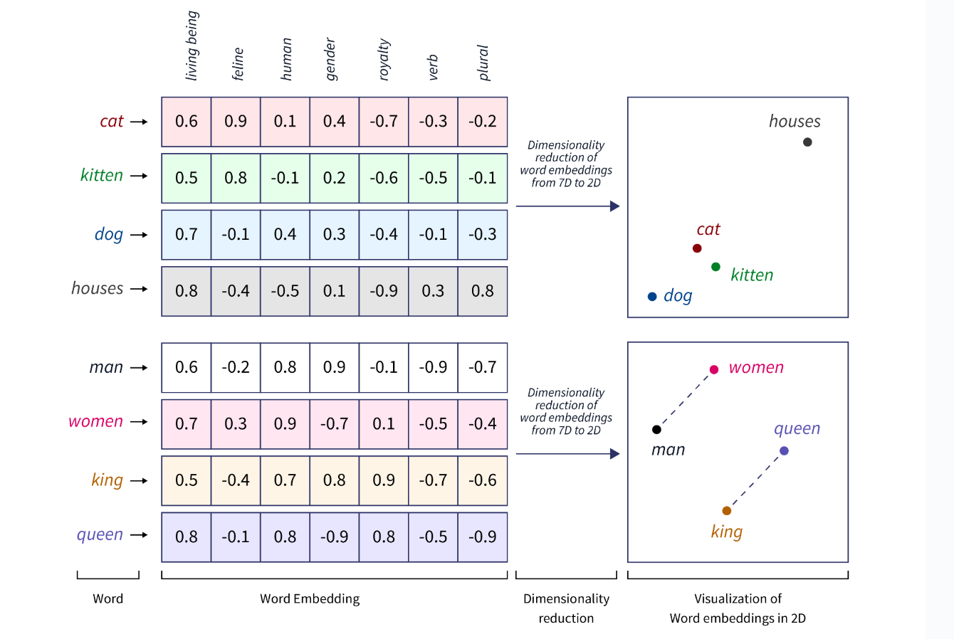
Word embeddings are featurized representations because the embeddings are n-dimensional vectors where each vector entry represents the value of a feature. For example, in the illustration above, the first vector entry is considered to represent the extent to which the object described by a word is a living being. When embeddings are learned, it may not be obvious what the feature represent.

Compared to traditional text representation approaches such as one-hot encoding, bag of words and TF-IDF, word embeddings have two main advantages:

• Word embeddings are dense vectors because the vector entries are real numbers. Hence, word embeddings solve the problem of sparsity found in other text representation approaches.
• Word embeddings are low dimensional representations created with deep neural networks, hence word embeddings address the issue of high dimensionality.
• Word embeddings are a distributed representation, meaning the vector space is dense and low dimensional.
• Word embeddings capture the context, semantic and syntactic similarity between words, providing richer information for training NLP models and achieving NLP tasks.
• For word embeddings, each dimension of the vector represents a feature or an aspect of the words meaning or context.
• Word embeddings are often used as input features into machine learning models for text classification, machine translation, named entity recognition, sentiment analysis, etc.

Word embeddings can improve the accuracy of machine learning models. Since word embeddings capture contextual information about words as well as semantic and syntactic similarity, word embeddings provide a richer representation of text than approaches such as one-hot encoding and bag-of word representations. Therefore, models trained with word embeddings performance better in NLP task such as text classification and named entity recognition and machine translation.

Properties of Word Embeddings

• Word context consists of the surrounding words or phrases that provide meaning and clarity to a specific word in a sentence. That is, nearby words that appear immediately before or after a target word make up a word context.
• Words that have a similar context are similar in meaning and have close vectors in the vector space.
• Word embeddings capture various semantic relationships between words, such as synonyms, antonyms, and analogies.
• Word embeddings allow for mathematical operations between word vectors, such as vector addition and subtraction. For example, a mathematical operation can be performed with the vectors for king, man, queen, and woman as follows:

\[man - woman = king - queen\] \[king - man + woman = queen\]

That means the distance between the vectors representing man and woman is approximately the same as the distance between the vectors king and queen. This mathematical operation was noticed with embeddings trained using word2vec. This amazing mathematics of computational linguistics reflects the analogy that man is to woman as king is to queen. Therefore, word embeddings can also help in building an analogy system.

When an embedding is learned for every word, the embeddings can be used for NLP modeling. For example, language models could be constructed to predict words given their context in a sentence. The embeddings of context words are used as input while the center or target word is used as output in the language model. Let’s examine how embeddings are learned.

Embedding Models

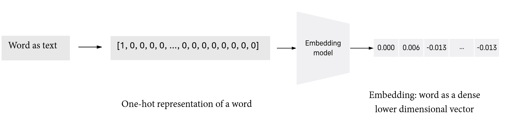
Embedding models are models that convert text corpora into dense and low dimensional vectors in a vector space. An embedding model takes an input text in the form of one-hot vectors and converts the one-hot encoding into embeddings. Below is an illustration of how an embedding model transforms a word represented as one-hot vector into an embedding.

There are several embedding models, however, an embedding model is generally a function that transforms an input text into an embedding (or a dense and low dimensional vectors in a numerical vector space). A simple embedding model or function multiplies a transposed VxN embedding matrix, \(W^T\) by a Vx1 one-hot vector, \(x\) to get an embedding vector, \(e\) for a word as shown below: \[W^Tx=e\]

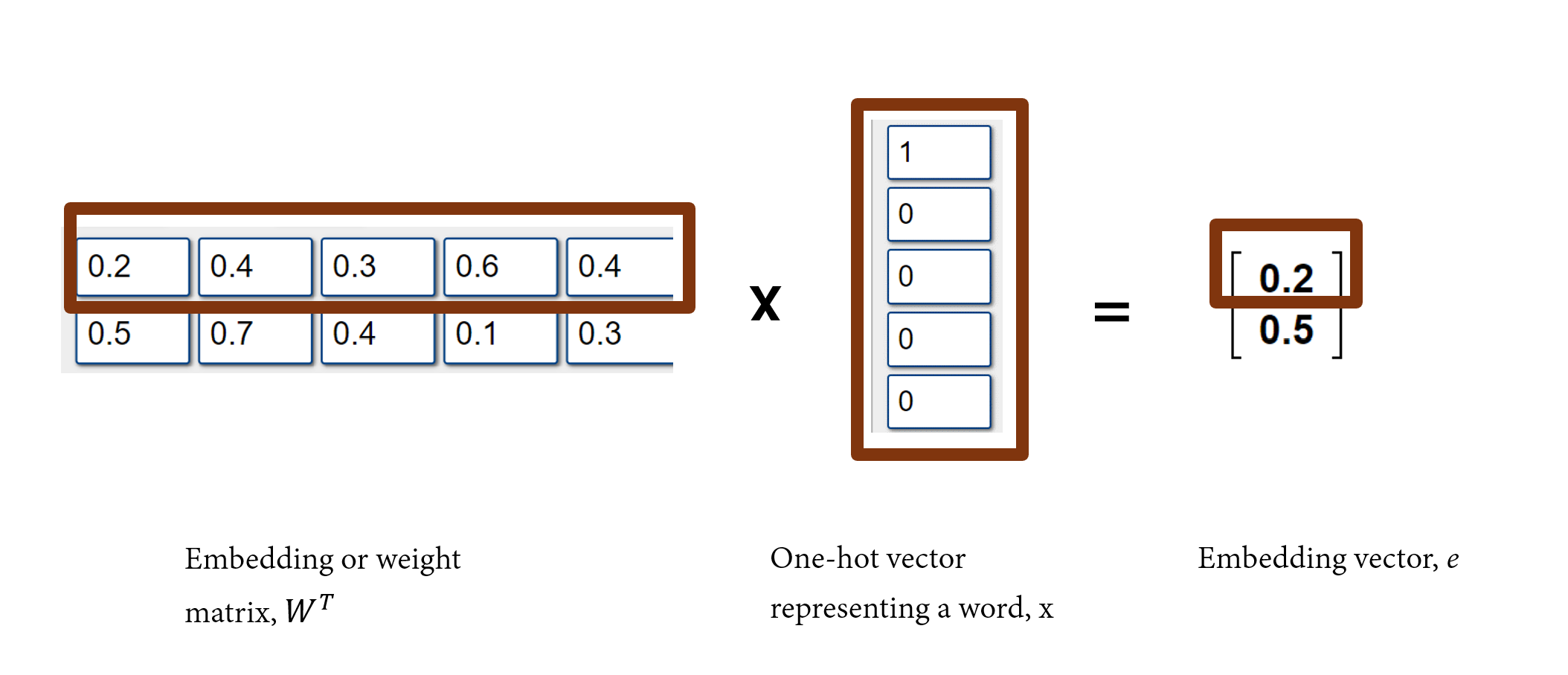
The embedding matrix can be viewed as a look up table. You would notice that if we multiply the embedding matrix by the one-hot vector of the jth word, we will get an embedding, which is the same as the jth column of the transposed embedding matrix, due to the zeros in one-hot vector.

So, we can view the embedding matrix as a look up table where the embedding vector of a word is simply retrieved from the look up table based on the position or index of the word. For example, the first column entries,[0.2, 0.5], of the transposed embedding matrix \(W^T\) would be retrieved for the one-hot vector [1, 0, 0, 0, 0]. Then, [0.4, 0.7] would be retrieved as the embedding for the word whose one-hot vector is [0, 1, 0, 0, 0]; and so on.

The embedding matrix used to transform one-hot encoded text into embedding vectors can also be viewed as weights. These weights can be learned using a neural network. For example, the embedding model, word2vec, is a neural networks that learns dense and low dimensional vector representation of text. Word2vec, GloVe and FastText are popular word embedding models for learning word embeddings.

Word2Vec

Word2vec is a neural network model trained with a language modeling objective. However, the ultimate goal of word2vec is to learn word embeddings. Neural word embeddings are generally trained with some sort of language modeling objectives such as predicting a missing word given surrounding words. Word2vec either predicts the probability of a target word in a vocabulary given some context words or predicts the probability of context words given a target word. There are two architectures for implementing Word2vec, known as, Continuous Bag of Words (CBOW) and Skip-gram, proposed by Google researchers (Mikolov, T. et. al) in 2013.

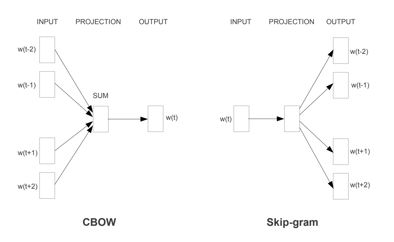
Continuous Bag of Word Model (CBOW)

CBOW is a neural network that learns word embeddings in the process of predicting the probability of a word given the context words, P(target word|context words). Predicting the probability of a word given it’s context is like trying to fill in the blank.

For example, the sentence “For God so loved the world that he gave his one and only Son, that whoever believes in him shall not perish but have eternal life.” could be written as “For God so loved the world that he gave his one and only ____, that whoever believes in him shall not perish but have eternal life.” Hence, the model can learn the embeddings in the text by finding the probability distribution of target words in the vocabulary given the context words.

Definitions of some terms

• A target word is a word in a sentence or text that is the focus of the analysis. The target word is also called the middle, current or center word.
• Context words are words that surround the center word.
• A context window is a range of context words surrounding a target word.
• A context window size or width is the number of context words to be considered on each side of the target word in a natural language modeling task.

How to create training samples for CBOW

When the context window size is defined, each word in the vocabulary is extracted as the target word and the corresponding context words surrounding each target word are also extracted. So, a training sample for a CBOW model is represented as a pair of context words and target word, (context, target).

General Training Sample for CBOW

For a sequence of words: \(w_1, w_2, w_3, ..., w_{t-m}, ..., w_{t-1}, w_t, w_{t+1}, ..., w_{t+m}, ..., w_{T-1}, w_T\), where \(w_t\) is the current target word, \(m\), the context window size, and \(T\), the number of training samples; Given a window size of m=2, the training sample can be generally written as: \[((w_{t-2}, w_{t-1}, w_{t+1}, w_{t+1}), w_t)\]

For example, given the text “Mary, did you know that your baby boy Would one day walk on water?”, the clean sequence of words without stop words would be:

['mary', 'know', 'baby', 'boy', 'would', 'one', 'day', 'walk', 'water'].

The training samples given a context window of size=2 can then be generated as follows:

Training Samples

((know, baby), mary),

((mary, baby, boy), know),

((mary, know, boy, would), baby),

((know, baby, would, one), boy),

((baby, boy, one, day), would), ...

In practice, the set of context words and target word pairs in the training data are represented by the indexes of the words in the vocabulary. The indexes of words are then used to retrieve the embeddings for the words. For example, the sample ((know, baby), mary) in the text above is represented as ((1, 2), 0).

The window size determines the span of context words on either side of a target word. Note that the context words surrounding the target words at the beginning or end of a sequence of words are truncated since the number of context words before or after the target words may be less than the context window size.

For example, the sample, ((know, baby), mary) is truncated as the window size of 2 should normally produce four context words. Since mary is the first word, there are no context words before mary, resulting to a truncated sample, ((know, baby), mary).

A CBOW architecture consists of the following layers:

1. An input layer:

• The input layer is made up of one-hot vectors of context words that surround the target word.
• The dimension of each context one-hot vector is Vx1, where V is the size of the vocabulary.
• In between the input layer and hidden layer is the input-hidden weight matrix.
• Each one-hot encoded context words is transformed by the same input-hidden weight matrix into context word embedding vectors. That is, the same input-hidden weight matrix is used as a look up table for retrieving context embeddings for the context words.
• These weight matrix represent the embeddings for the context words.

2. A hidden layer:

The hidden layer is the computational unit that transforms each one-hot context vector using the same input-hidden weight matrix into a context word embedding as shown below.

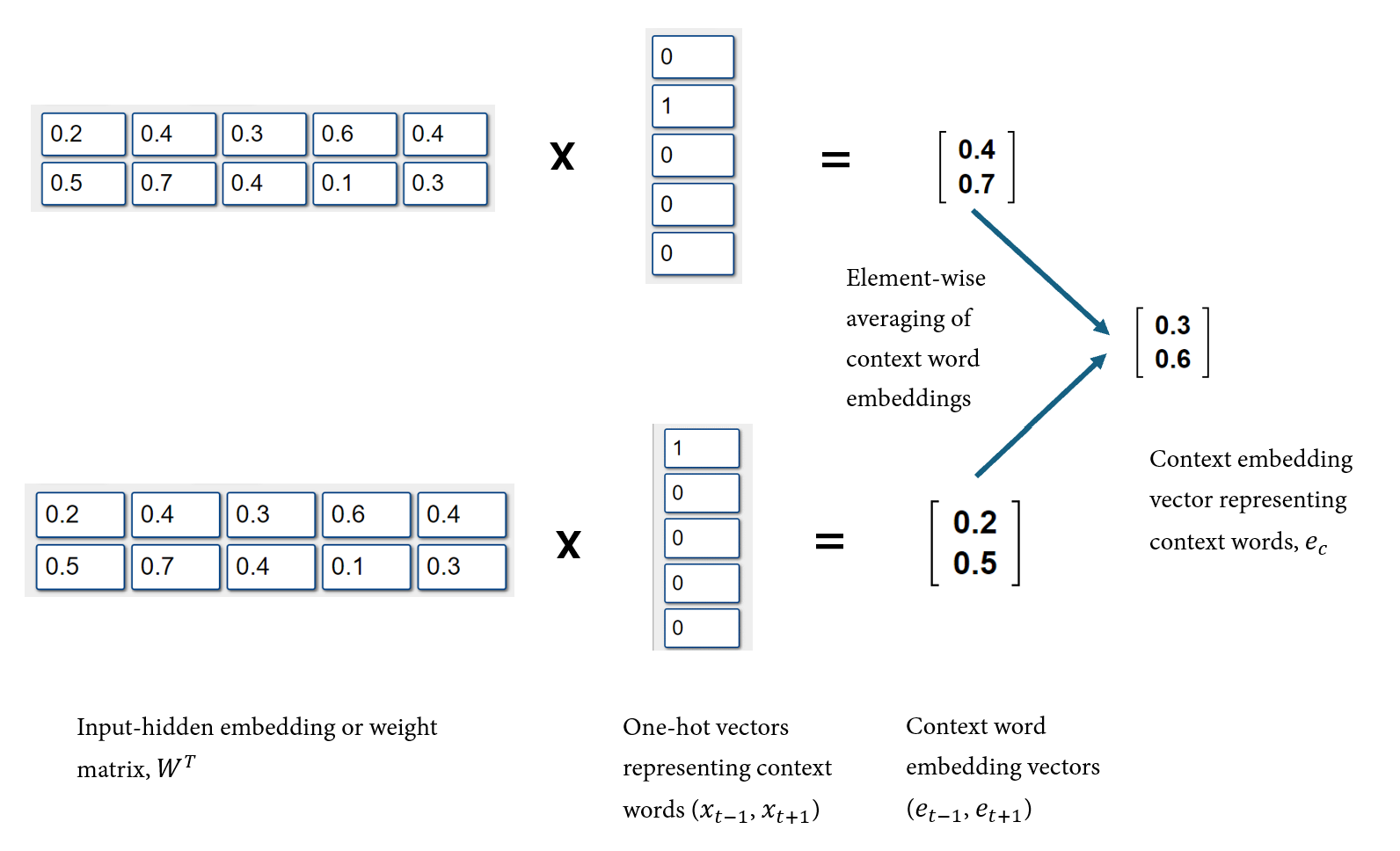
• Mathematically, a VxN input-hidden weight matrix, \(W\), is transposed and multiplied by each Vx1 one-hot context word vector to get each Nx1 context word embedding vector, where V is the vocabulary size and N is the number of nodes in the hidden layer or the dimension of the context embedding vectors.
• In practice, the embedding matrix or input-hidden weight matrix is used to look up the embeddings of the context words.
• The Nx1 context word embedding vectors are then combined through an element-wise averaging operation to get a shared Nx1 context embedding vector, \(e_c\), that represents the context words associated with the target word, \(t\). That is, \(e_c = \frac{1}{2m}(e_{c1} + e_{c2} + e_{c2m} +...)\); where 2m = number of context words in the defined context window (m=window size).
• Hence, considering all the target words in a text corpus, the hidden layer can be viewed as a shared projection layer that projects high dimensional input context words into a shared vector space (shared projection matrix). There is no activation function in the hidden layer.

3. An output layer:

• The softmax output layer transforms the shared context embedding vector using a hidden-output weight matrix and a softmax function to produce probability distribution of vocabulary words given the context, \(P(word/context)\) as shown below.

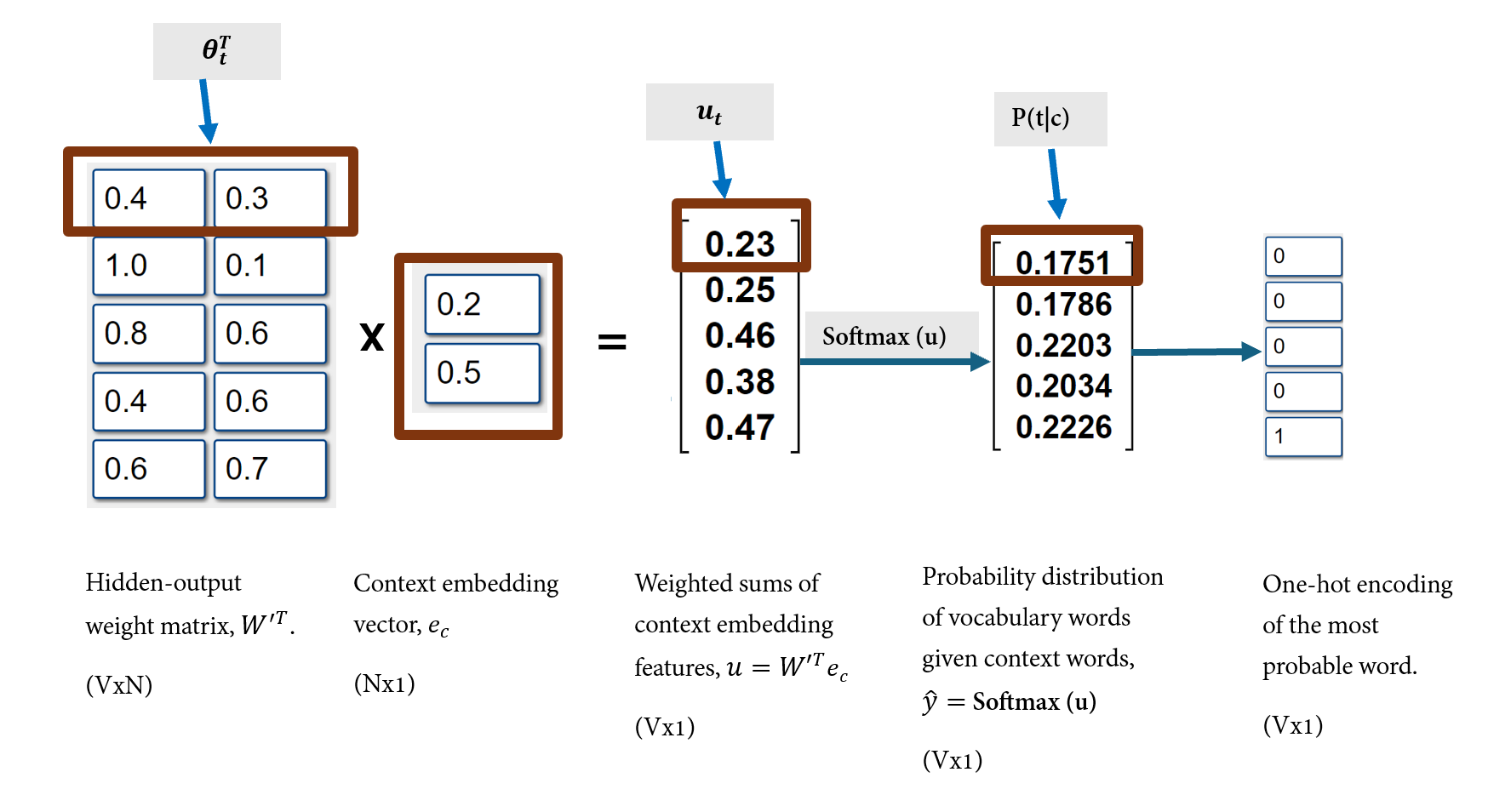
• In the output layer, the transposed hidden-output weight matrix \(W'^T\) and shared context embedding vector \(e_c\) are multiplied to obtain a vector, \(u = W'^Te_c\).

• The \(jth\) entry, \(u_j\) of the vector \(u\) is associated to the \(jth\) word in the vocabulary. \(u_j\) can be viewed as dot product of the \(jth\) column of \(W'\), denoted \(\theta_j\) and the context embedding vector, \(e_c\): \(u_j = \theta^T e_c\).

• The dot product can also be viewed as a weighted sum of the context embedding vector where the weights applied are entries of \(\theta_j\). For example:

\[\begin{align} \theta^T &= \left[\begin{array}{cc} 0.4 & 0.3\\ \end{array}\right] \\ e_c & = \left[\begin{array}{cc} 0.2 \\ 0.5 \end{array}\right] \\ \\ u_j &= \theta^T e_c \\ & = 0.4*0.2 + 0.3*0.5 \\ & = 0.23 \end{align}\]

Softmax Function for CBOW

The probability of a target word given context words is calculated using using the softmax function as:

\[\begin{align} P(t|c) &= Softmax(u_t) \\ &= \frac{exp({u_t})}{\sum_{j=1}^{V}{exp({u_j})}} \\ &= \frac{exp({\theta^T_t e_c})}{\sum_{j=1}^{V}{exp({\theta^T_j e_c})}} \end{align}\]

Where:

• \(u_t\) is a scalar input of the softmax function associated with the target word, \(t\), whose probability is being estimated.
• \(u_j\) is a scalar input of the softmax function for the jth word in the vocabulary; \(j = {1, 2, 3, ..., V}\).
• \(e_c\) is the given input context embedding word vector.
• \(\theta_j\) is an Nx1 vector equivalent to jth column of \(W'\). \(\theta_j\) is associated with the jth vocabulary word while \(\theta_t\) is associated with the current target word in the vocabulary.

The loss function of the CBOW model

The loss function captures the performance of the model. For a CBOW model, the cross-entropy is typically used for the loss function. Since the CBOW model predicts the probability distribution of vocabulary words given the context words, where the vocabulary words can be treated as classes, the CBOW model can then be viewed as a model that achieves a multi-class classification task.

Loss Function for CBOW

The cross-entropy loss function, denoted \(l(y, \hat{y})\) or \(J(\theta)\) for a single training sample for CBOW is written as:

\[\begin{align} l(y, \hat{y}) &= - y_j \log{\hat{y_j}} \\ J(\theta) &= - y_j \log{\frac{exp({\theta^T_t e_c})}{\sum_{j=1}^{V}{exp({\theta^T_j e_c})}}} \end{align}\]

Where:

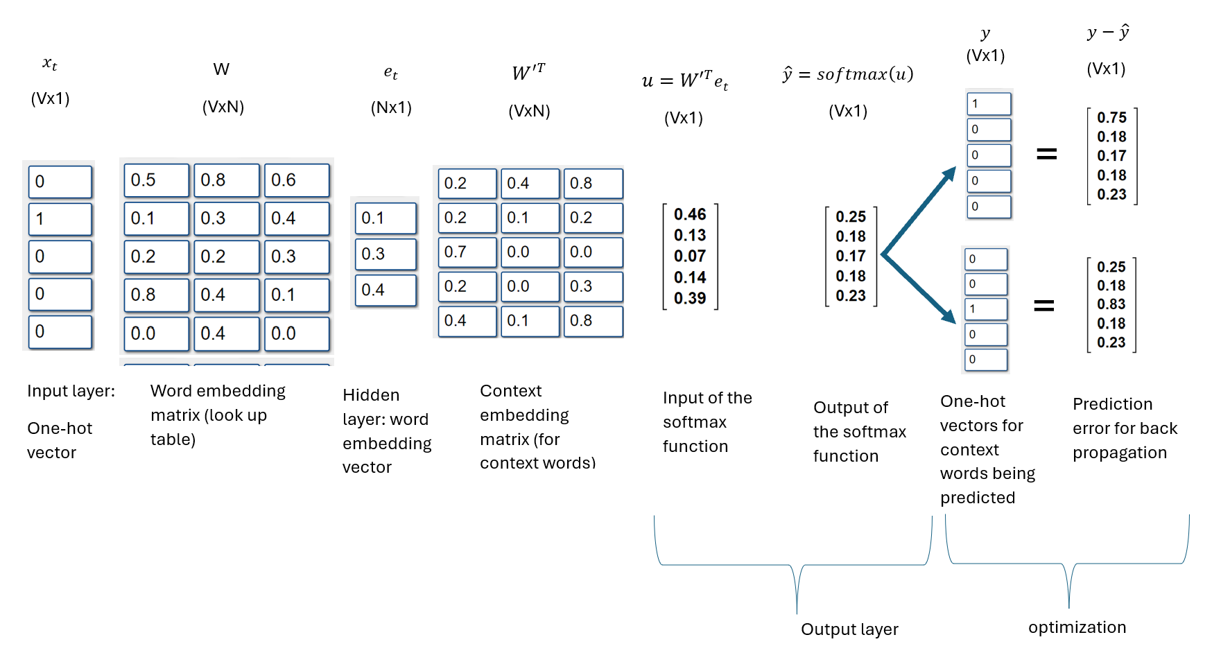
• \(y\) is a one-hot vector of the actual target word,
• \(\hat{y}\) is the vector representing the output of the softmax function, \(\hat{y} = softmax(u)\).
• \(\hat{y_j}\) and \(y_j\) are the jth values of the \(\hat{y}\) and \(y\) vectors respectively.

CBOW model optimization

The computed loss \(J(\theta)\) is used for back propagation to update the weight matrices, \(W\) and \(W'\). Specifically, the partial derivatives of the loss function with respect to each parameter in the loss function are used in a stochastic gradient descent (SGD) rule to update the parameters iteratively.

During each SGD iteration, a single training example is used to update the weights or parameters, \(\theta = \{\theta_j, \ e_{ci} \}\), of \(J(\theta)\).

where:

• \(\theta_j\) represent all the vectors or columns in the hidden-output weight matrix \(W'\).
• \(e_{ci}\) represents all the embedding vectors of the context words associated with the current target word. The context word embedding vectors \(e_{ci}\) are rows of the input-hidden weight matrix, \(W\), representing the context words surrounding the current target word.

Recall that the average context word embedding, \(e_c = \frac{1}{2m}(e_{c1} + e_{c2} + e_{c3}...,e_{c2m})\); m = context window size and 2\(m\) = number of context words in the context window.

Stochastic Gradient Descent Optimization for CBOW

The following gradient descent rule is used to update the parameter \(\theta\) for a single training sample during each SGD iteration:

\[ \theta_j = \theta_j - η\frac{\partial J(\theta)}{\partial \theta_j}; \text{ where } j = {1, 2, 3, ..., V}\]

\[ e_{ci} = e_{ci} - η\frac{\partial J(\theta)}{\partial e_{ci}}; \text{ where } i = {1, 2, 3, ..., 2m}\]

The average context word embedding vector \(e_c\) was used to compute the output of the softmax function, however, in back propagation, we are updating the individual context embedding vectors or columns of input-hidden weight matrix, \(W\). You can view the average context word embedding vector as an approximation of each context vector used to obtain the average context word embedding vector.

Note

The ultimate goal of training a CBOW model is to learn the embedding matrix, \(W\), which is a vector space model or a collection of dense and lower dimensional vector representation of the words in the vocabulary.

CBOW vs language model

The CBOW is similar to a language model but they are slightly different. CBOW and language models both predict the probability of a target word given context words. CBOW and language models are different in that, the context words for CBOW are words before and after the target word within a context window but the context words in language models are words that precede the target word. The order of words do not matter in CBOW compared to language models where the order of words matter.

Continuous Skip-gram Model

Skip-gram is another word2vec architecture for learning word embeddings. A skip-gram model learns word embeddings by predicting the probability distribution of context words given a target word. Skip-gram is opposite to CBOW: CBOW computes P(target word|context) while skip-gram computes P(context|target word).

How to create the training samples for skip-gram

The text data used to train a skip-gram model consists of a collection of input target words and output context words within a defined context window. That is, the training sample is a (target_word, context_words) pair. If the position of a target word is t, and the context window size is 2, then, we can estimate the probability of all context words given the target word through forward propagation while maximizing the probability of context words at location (t-2), (t-1), (t+1) and (t+2) through back propagation.

Given the text “Mary, did you know that your baby boy Would one day walk on water?”, we get the vocabulary of words: ['mary', 'know', 'baby', 'boy', 'would', 'one', 'day', 'walk', 'water'].

The training samples for a context window size of 2 can then be generated as follows:

Training Samples

(mary,know),

(mary, baby),

(know, mary),

(know, baby),

(know, boy), ...

We can notice from the training examples that skip-gram does not predict all the context words at once but predicts each context word in the context window given the target word. Hence, skip-gram captures the context words for each target word using multiple training examples.

Skip-gram architecture

A skip-gram architecture consists of the following layers:

The skip-gram model structure is as follows:

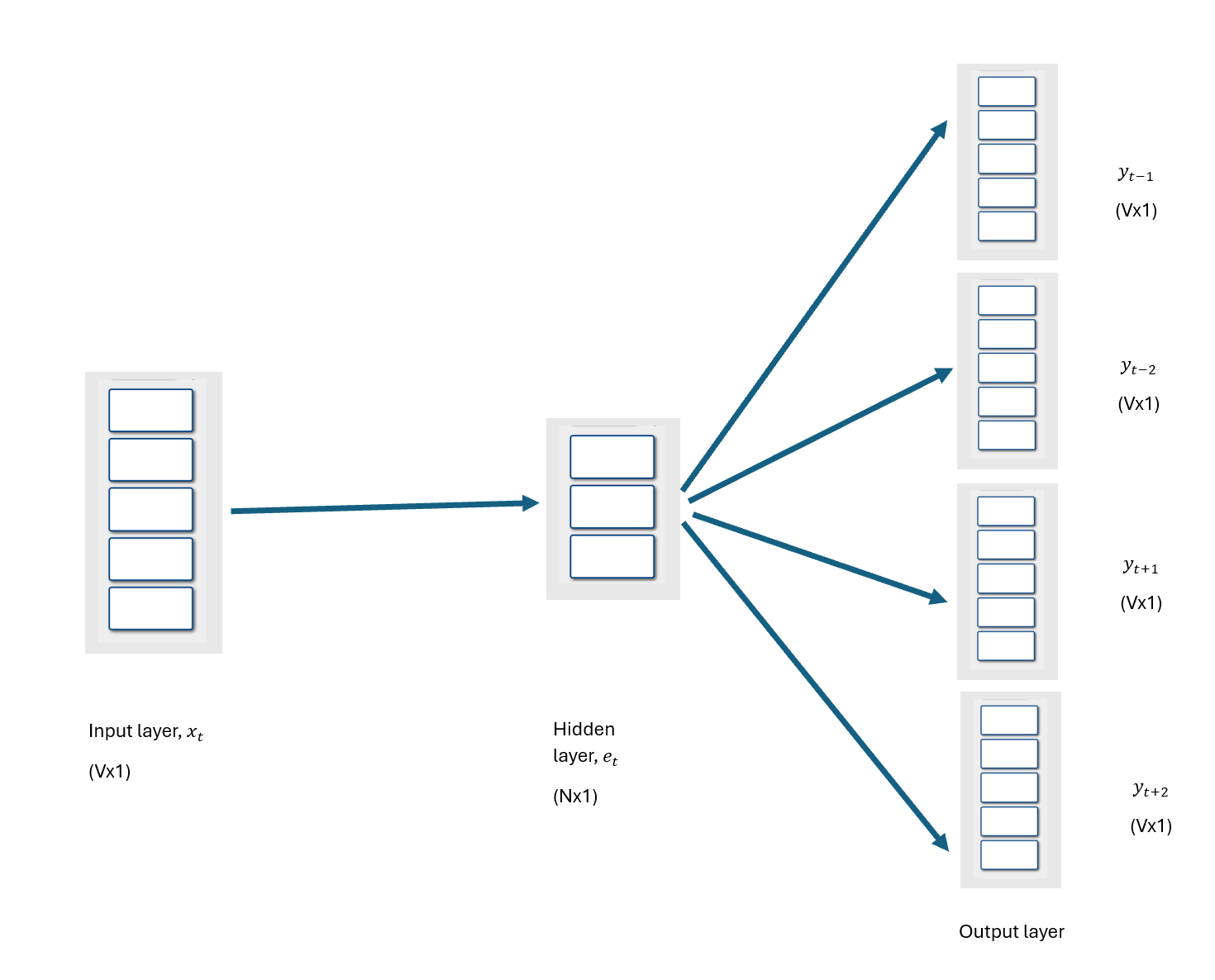
1. An input layer:

• The input layer is a Vx1 one-hot vector \(x_t\), representing the target word in a vocabulary of size V.
  
• In between the input layer and hidden layer is a VxN input-hidden weight matrix \(W\), also known as the word embedding matrix; V = vocabulary size, and N = number of nodes in the hidden layer.
• The one-hot encoded word \(x_t\) in the input layer is transformed by the input-hidden weight matrix \(W\) to produce an Nx1 word embedding vector \(e_t\), a dense vector representing the target word.

2. The hidden layer:

• The hidden layer is a computational unit that multiplies the NxV matrix \(W^T\) by the Vx1 one-hot word vector \(x_t\) to produce an Nx1 word embedding vector \(e_t\) for the target word. That is, \(W^Tx_t = e_t\). There is no activation function in the hidden layer.
• In practice, the hidden layer basically uses the index of the word represented by the one-hot vector to look up the word embedding vector \(e_t\) in embedding weight matrix, \(W\). The jth column of the NxV matrix \(W^T\) is the word embedding for the jth word in the vocabulary.
• There is an NxV context embedding matrix \(W'\) between the hidden layer and the output layer. \(W'\) is used to transform the word embedding vector \(e_t\).

3. The output layer:

• The output layer is also called the softmax output layer because this layer uses a softmax activation function to generate a probability distribution of context words given a target word.
• In the output layer, the word embedding vector \(e_t\) of the target word is multiplied by the transposed context embedding matrix \(W'^T\) to obtain the Vx1 vector \(u\) as follows: \[u=W'^Te_t\]
• The \(jth\) column of \(W'\) is an Nx1 context word embedding vector \(\theta_j\) for the \(jth\) word in the vocabulary, with dimension Nx1. The dot product of \(\theta^T_j\) and \(e_t\) gives the \(jth\) entry \(u_j\) of vector \(u\), where j={1, 2, 3, … V}.

\[u_j=\theta_j^T e_t\]

Softmax for Skip-gram

The probability of a context word given the target word is calculated using using the softmax function as follows: \[\begin{align} Softmax(u_c) &= P(c|t) \\ &=\frac{exp({u_c})}{\sum_{j = 1}^{V}{exp({u_j})}} \\ Softmax(\theta_c^T e_t) & = \frac{exp({\theta_c^T e_t})}{\sum_{j = 1}^{V}{exp({\theta_j^T e_t})}} \end{align}\]

Where:

• \(c\) is the context word whose probability is being estimated.
• \(t\) is the given target word associated with the context word.
• \(u_c\) is the scalar input of the softmax function associated with the context word \(c\), whose probability is being estimated.
• \(u_j\) is the scalar input of the softmax function for the jth context word in the vocabulary, where j={1, 2, 3, …, V}.
• \(\theta_c\) is the context word embedding vector for the context word \(c\).
• \(\theta_j\) is the context word embedding vector for the jth context word in the vocabulary, where \(j={1, 2, 3, ..., V}\).

Note

The context words share the same output layer, hence the output of the softmax is a vector:

\[\begin{align} \hat{y} &= \left[\begin{array}{cc} P(c_1/t) \\ P(c_2/t) \\ P(c_3/t) \\ . \\ . \\ . \\ P(c_V) \end{array}\right] \end{align}\]

where \(c_j\) is the jth word (context word) in the vocabulary of size V, and t, the target word.

Though the output of the softmax function estimated during forward propagation share the same output layer, only the joined probability of context words associated with the current target word is maximized during each back propagation step.

Training the skip-gram model

The skip-gram model is trained through forward and backward propagation. Forward propagation computes the probability distribution of vocabulary word given the target word while backward propagation computes the errors and updates the weights to minimize the prediction errors (or maximize the joined probability of context words given the target word).

The training objective of the skip-gram model is to maximize the probability of predicting context words given the target word. That is, during training, we want to find the parameters or weights of the embedding matrices that result to the highest probability for the context words given the target word.

If the context words \(c_1, c_2, c_3,... c_4\) are observed around the target word \(t\), then, we can maximize the probability of the context words appearing together given the target word: \(\text{maximize }P(c_1, c_2, c_3, c_4|t; \theta)\)

Skip-gram Model Objective

For a sequence of words \(w_1, w_2, w_3, w_3, ..., w_{t-m}, ..., w_{t-1}, w_t, ..., w_{t+m}, ..., w_{T-1}, w_T\), the objective of the skip-gram model is to: \[\text{maximize }P(w_{t-m}, ..., w_{t-1}, w_t, ..., w_{t+m}|w_t)\]

where:

• \(w_t\) is the current target word
• \(m\) is the context window size;
• \(T\) is the number of training samples;

The joined probability of context words given a target word within a single window is computed using the softmax function, which takes a dot product of the word embedding vector \(e_t\) and context word embedding vector \(\theta_c\) as input.

These dot products measure similarity, so maximizing the probability of context words given the target word in a window is the same as maximizing similarity between \(e_t\) and \(\theta_c\).

Skip-gram Objective Function for a Batch Gradient Descent

Mikolov et al.(2013) in their paper, Distributed Representations of Words and Phrases and their Compositionality, stated the objective function for batch gradient descent for the skip-gram model as:

\[J(\theta)=-\frac{1}{T}\sum_{t = 1}^{T}\sum_{-c \le j \le c, j \neq 0}\log{p(w_{t+j} | w_t)} \] This cost function maximizes the average probability of the context words given a target word across all windows for each iteration of the gradient descent algorithm by:

• finding the joined probability of context words given a target word within each window,
• finding the average of all the joined probabilities,
• finding the parameter settings that produce the highest average joined probability of context words given a target word.

Maximizing the probability of context words given a target word in a window is the same as finding the parameters of the word embedding vector and context word embedding vector with the highest probability of context words appearing near the given target.

So, to maximize the joined probability of context words given a target word within a window, only context word embedding vectors for context words and word embedding vector for the target word within that window are updated.

Hence, for a batch gradient where the objective is to maximize the average probability of context words given the target word across all windows; all word embedding vectors and all context word embedding vectors across windows need to be updated. This is computationally expensive and impractical because of too many gradients are computed to update all of the parameters in the model in a single iteration.

To solve this issue of computing gradient for too many parameters in a single iteration, stochastic gradient descent can instead be used to update parameters only within a single window during each iteration.

Skip-gram Objective Function for Stochastic Gradient Descent

For a stochastic gradient descent, the objective of the Skip-gram model is to maximize the joined probability of context words given the target word within a window as follows:

\[\begin{align} P(c/t) &= P(w_{t-m}, ..., w_{t-1}, w_t, ..., w_{t+m}|w_t) \\ &= P(w_{t-m}|w_t)...P(w_{t-2}|w_t)P(w_{t-1}|w_t)P(w_{t+2}|w_t)...P(w_{t+m}|w_t) \\ &= \prod_{-m \le i \le m, i \neq 0} P(w_{t+i}|w_t) \\ &=\prod^{C}_{c=1} \frac{exp({\theta_c^T e_t})}{\sum_{j = 1}^{V}{exp({\theta_j^T e_t})}} \end{align}\]

where:

• \(c\) = number of context words
• \(m\) = context window size

Therefore, the Skip-gram cost function we want to maximize for a single window or target word is as follows:

\[ J(\theta)_{maximize} =\prod^{C}_{c=1} \frac{exp({\theta_c^T e_t})}{\sum_{j = 1}^{V}{exp({\theta_j^T e_t})}} \]

Maximizing a function is the same as minimizing the negative of the function, hence we can formulate the cost function for Skip-gram as a minimization problem as follows:

\[ J(\theta)_{minimize} = -\prod^{C}_{c=1} \frac{exp({\theta_c^T e_t})}{\sum_{j = 1}^{V}{exp({\theta_j^T e_t})}} \]

Gradient descent optimization requires the derivative of the cost function. However, it is mathematically easier to find the derivative of a sum than the derivative of a product. Therefore, we will apply log to the cost function to simplify the cost function into an addition problem.

Applying log does not affect the optimized weights (θ) because natural log is a monotonically increasing function. That is:

\[ J(\theta)_{minimize} = \log{J(\theta)_{minimize}} \]

Cost Function for Maximizing the Probability of Context Words given the Target Word

The Skip-gram cost function for maximizing the probability of context words given a target word in a window can be written as:

\[\begin{align} J(\theta) &= - \log{ \prod^{C}_{c=1} \frac{exp({\theta_c^T e_t})}{\sum_{j = 1}^{V}{exp({\theta_j^T e_t})}}} \\ &= - \sum^{C}_{c=1} \log{ \frac{exp({\theta_c^T e_t})}{\sum_{j = 1}^{V}{exp({\theta_j^T e_t})}}} \\ &= - \sum^{C}_{c=1}\theta_c^T e_t + C\log{\sum_{j = 1}^{V}{exp({\theta_j^T e_t})}} \end{align}\]

Gradient of Skip-gram Cost Function

Word and Context Embedding Vectors

Every vocabulary word is represented in a Skip-gram model as a word embedding vector and context embedding vector. That is, the jth word in the vocabulary is represented as:

• \(e_j\), the word embedding vector equivalent to the jth column of the VxN word embedding matrix \(W\).
• \(\theta_j\), the context word embedding vector equivalent to the jth column of the NxV word embedding matrix \(W'\).

For a stochastic gradient descent the following parameters of the model are updated within a window for each iteration:

• the weights in the word embedding vector \(e_t\) for the current target word.
• the weights in the context word embedding vectors, \(\theta_1, \theta_2, \theta_3, ..., \theta_C\) representing the context words of the current target word. Let’s use \(\theta_c\) denote any context word vector for a context word of the current target word.

Recall

The Skip-gram cost function to maximize the probability of context words given a target word can be written as:

\[ J(\theta)_{minimize} = - \sum^{C}_{c=1}\theta_c^T e_t + C\log{\sum_{j = 1}^{V}{exp({\theta_j^T e_t})}} \]

Gradient with Respect to the Word Embedding Vector

It can be shown that:

The gradient of the cost function with respect to the word embedding vector \[\begin{align} \partial J (\theta){\partial e_t} &= - \sum^{C}_{c=1}\theta_c^T + C\sum^{V}_{k=1} \frac{exp({\theta_k^T e_t})}{\sum_{j = 1}^{V}{exp({\theta_j^T e_t})}} \\ &= - \sum^{C}_{c=1}\theta_c^T + C\sum^{V}_{k=1} P(k|t)\theta_k \end{align}\]

where:

• t is the target word for the current window.
• k is any word (context) in the vocabulary and
• \(C\) = number of context words in the current window.

Gradient with Respect to Context Word Embedding Vectors

The gradient of the cost function with respect to a context word embedding vector representing a context word within a context window is as follows:

\[\begin{align} \partial J (\theta){\partial \theta_c} &= - e_t + C\frac{exp({\theta_c^T e_t})}{\sum_{j = 1}^{V}{exp({\theta_j^T e_t})}} \\ &= - e_t + C\ P(c|t)e_t \end{align}\]

where:

• \(c\) is any context word in the current window.
• t is the target word for the current window.
• \(C\) = number of context words in the current window.

Stochastic Gradient Descent Optimization for Skip-gram

The following general gradient descent rule is used to update the parameter \(\theta\) for a single iteration:

Update the weights in word vector of current target word

\[\begin{align} e_t &= e_t - η\frac{\partial J(\theta)}{\partial e_t} \end{align}\]

Update the weights in context word vectors of current target word \[\begin{align} \theta_c &= \theta_c - η\frac{\partial J(\theta)}{\partial \theta_c} \\ \text{ where } c &= {1, 2, 3, ..., C} \end{align}\]

Optimization Using a Training Sample in each Iteration

So far, we have discussed SGD optimization where the probability of context words in a context window given a target word is maximized by optimizing the cost function:

\[ J(\theta)_{minimize} = - \sum^{C}_{c=1}\theta_c^T e_t + C\log{\sum_{j = 1}^{V}{exp({\theta_j^T e_t})}} \] This cost function is used when each iteration of the SGD optimization focuses on maximizing the probability of context words occurring together given a target word within a context window. This explains why we sum from c=1 to C in the cost function.

Note

However, in practice, the probability of a single context word given a target word in a window is maximized during each SGD iteration. This is a simplified skip-gram optimization where the parameters of only one context word vector and one word embedding vector are updated in each SGD iteration.

Suppose a window has C context words, then C training sample pairs are generally obtained for each window.

The cost function for maximizing the probability of each context word given a target word in a window during each SGD iteration is:

Cost Function to Maximize \(P(\text{one context word | target word})\)

\[\begin{align} J(\theta)_{maximize} &= P(\text{context word|target word}) \\ J(\theta)_{maximize} &= \log{ \frac{exp({\theta_c^T e_t})}{\sum_{j = 1}^{V}{exp({\theta_j^T e_t})}}} \\ J(\theta)_{minimize} &= - \log{ \frac{exp({\theta_c^T e_t})}{\sum_{j = 1}^{V}{exp({\theta_j^T e_t})}}} \\ &= - \theta_c^T e_t + \log{\sum_{j = 1}^{V}{exp({\theta_j^T e_t})}} \\ \end{align}\]

Hence the gradients of the cost function for maximizing the probability of each context word given a target word in a window during each SGD iteration with respect to the word embedding vector and context word embedding vector is as follows.

## Gradient of Cost Function to Maximize \(P(\text{one context word | target word})\)

\[\begin{align} \partial J (\theta){\partial e_t} &= - \sum^{C}_{c=1}\theta_c^T + \sum^{V}_{k=1} \frac{exp({\theta_k^T e_t})}{\sum_{j = 1}^{V}{exp({\theta_j^T e_t})}} \\ &= - \theta_c^T + \sum^{V}_{k=1} P(k|t)\theta_k \end{align}\]

\[\begin{align} \partial J (\theta){\partial \theta_c} &= - e_t + \frac{exp({\theta_c^T e_t})}{\sum_{j = 1}^{V}{exp({\theta_j^T e_t})}} \\ &= - e_t + \ P(c|t)e_t \end{align}\]

These gradients are then used in the SGD rule to update the context word embedding and word embedding vectors representing the current context and target word.

Optimization Effeciency

During the optimization of a Skip-gram model, finding the sum in the denominator of the softmax function when computing the gradients is still computationally expensive, so other methods such as negative Skip-gram and hierarchical softmax are used to improve computational efficiency.

Skip-gram with Negative Sampling

This is basically a skip-gram model structure that uses a signmoid function in the output layer instead of a softmax function. The goal of the skip-gram with negative sampling is to learn embeddings by predicting whether a word is a context word or not given a target word.

The training data is created such that:

• for each target word in a window, (target, context) positive samples are generated by paring the target word with its context words.
• negative samples are created by pairing the target words with randomly select k words outside the context window of the target. Some probability distribution is used to randomly select k words outside the context window.
• for each positive pair (y=1), we sample k negative pairs (y=0).

Skip-gram with Negative Sampling Cost Function

We want to maximize the probability that the positive pairs occur together while also maximizing the probability that the negative pairs do not occur together.

For a positive sample pair the probability that they occur together is written as: \[P(y=1|t,c) = \frac{1}{1 + exp(-\theta^T_c e_t)}\] For a negative sample pair the probability that the target word and context word occur do not occur together is written as: \[P(y=0|t,c) = 1- P(y=1|t,c_k) = 1 - \frac{1}{1 + exp(-\theta^T_k e_t)} \]

The logistic or sigmoid function is used as the objective function since the problem is formulated as a classification problem.

For each training sample, the sigmoid function takes a scalar value obtained from the dot product of the context word embedding vector and word embedding vector as input.

For a single positive pair and k negative pairs, the objective function maximizes the probability of the positive pairs occurring together while also maximizing the probability of the negative pairs not occurring together.

The cost function for a Skip-gram with negative sampling for each positive pair and it’s corresponding sampled K negative pairs outside the window is formulated as follows:

\[\begin{align} J(\theta)_{maximize} &= P(y=1|t,c) \prod_{k = 1}^{K} (1 - P(y=1|t, c_k)) \\ &= P(y=1|t,c) + \sum_{k = 1}^{K} (1 - P(y=1|t, c_k)) \\ &= \log{P(y=1|t,c)} + \sum_{k = 1}^{K} \log{(1 - P(y=1|t, c_k))} \\ J(\theta)_{minimize} &= - \log{P(y=1|t,c)} - \sum_{k = 1}^{K} \log{(1 - P(y=1|t, c_k))} \\ &= - \log{\sigma(\theta^T_c e_t)} - \sum_{k = 1}^{K} \log{\sigma(-\theta^T_k e_t)} \end{align}\]

where:

• c is any positive context word for the current target word t.
• k is any negative context words for the current target word t.
• Total number of negative words is K.

This cost function is more computationally efficient to optimize than the softmax cost function.

GloVe

GloVe stands for Global Vector Word Representation.The GloVe algorithm was created by team of researchers from Stanford University, led by Jeffrey Pennington, Richard Socher, and Christopher D. Manning. They introduced the GloVe model in their paper titled “GloVe: Global Vectors for Word Representation,” which was published in 2014.

The GloVe algorithm is not popularly used as word2vec but it is simple and fast. GloVe learns word embeddings that capture semantic meaning of words and relationships between words using the global statistics (co-occurrence statistics) of words in a large corpus of text.

Word occurrence statistics is used by all unsupervised approaches for learning word embeddings in a corpus as the primary source of information available. For example, a word2vec Skip-gram model captures co-occurrences within a window at a time, while Glove captures co-occurrences globally, across the entire corpus.

GloVe allows us to understand how words embeddings capture the meaning of words from word occurrence statistics.

GloVe constructs a word-word co-occurrence matrix where each element \(X_{ij}\) of the co-occurrence matrix represents how often word \(j\) appears in the context of word \(i\) within a fixed window.

Below is an example of a term co-occurrence matrix.

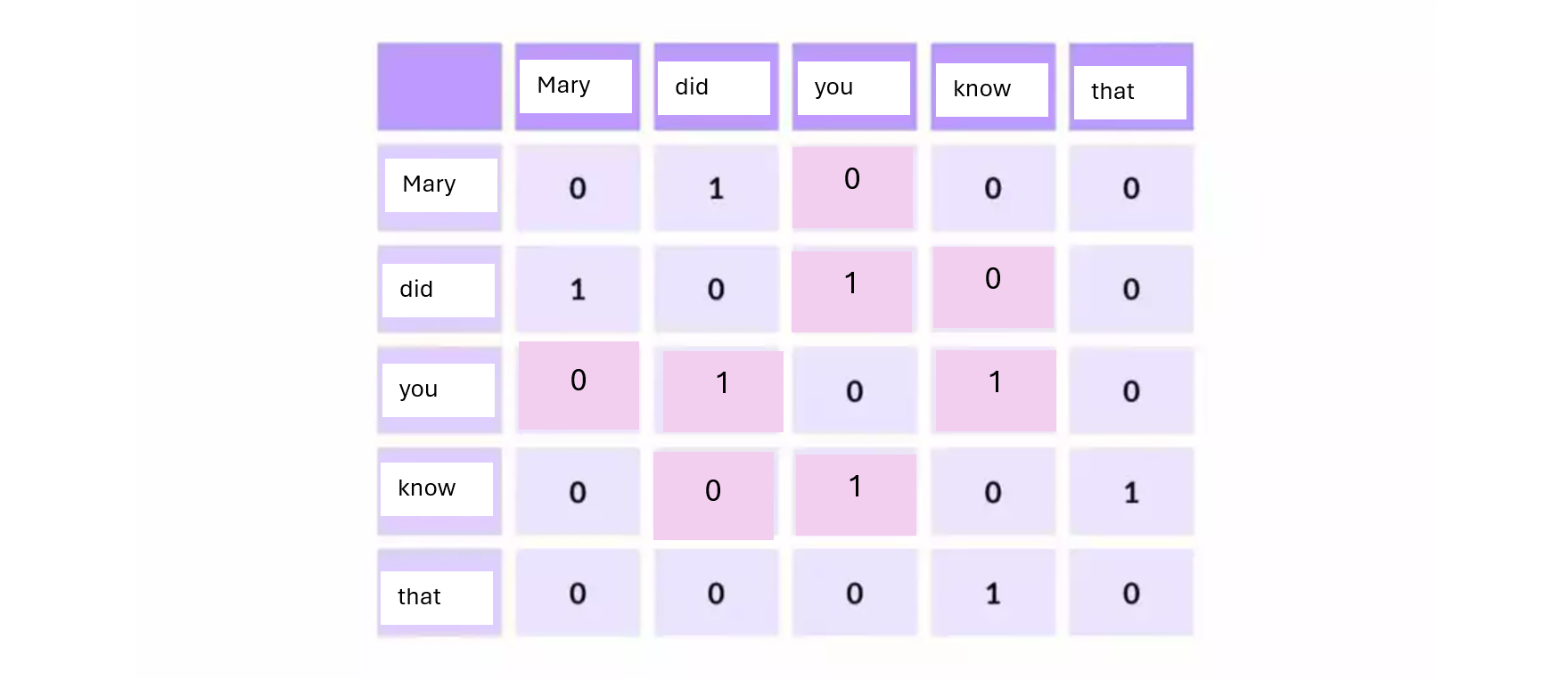
The co-occurrence matrix tabulates how frequently words co-occur with one another in a given corpus. The co-occurrence matrix can be very sparse and needs to be transformed into a dense lower dimensional representation.

A statistical approaches such as matrix factorization (for example, Singular Vector Decomposition or SVD) could be used to decompose the co-occurrence matrix into a \(USV^T\) decomposition, where the rows of \(U\) are the embedding vectors for words.

SVD is fast to implement with a small text corpus, and computationally expensive when the size of the co-occurrence matrix is large (such as when the vocabulary consists of millions of words). Additionally, it is hard to incorporate new words as this requires the SVD to be implemented again.

Co-occurrence Probability

The co-occurrence probability is denoted \(P_{ij}\) or \(P(i|j)\) is the probability of word \(j\) occurring in the context of word \(i\): \[P_{ij}=P(i|j)=\frac{X_{ij}}{X_i}\] where

• \(X_{ij}\) = the number of times word j occurs in the context of word i.
• \(X_i\) = the number of times word i occurs in the entire corpus.

Traning a Glove Model

Apart from using statistical approaches such as SVD to learn embeddings from the co-occurrence matrix, stochastic gradient descent can be used to train a GloVe model.

The training objective of GloVe is to learn word vectors by minimizing the the square of the difference between the dot product of word vectors and the logarithm of the words’ probability of co-occurrence.

The model needs to be train such that the dot product of the word and context vectors approximate the co-occurrence probability of the words. That is, the goal is to learn the parameters of a log-bilinear model: \[w_j^T\tilde{w_j}=\log{(P(i/j)})\]

In the nutshell, GloVe is a log-bilinear model with a least square objective.

• The dot product of a target word vector \(w_j\) and context word vector \(\tilde{w_i}\) represents the similarity between the target and context words. The higher the dot product, the greater the similarity between the words.
• The co-occurrence probability of words also capture information about the relationship between the words. Words that co-occur more frequently have a higher co-occurrence probability, which indicates a stronger relationship between words.

Hence, the objective of GloVe is to minimize the cost function:

\[\begin{align} J(\theta) &= \sum_{i,j=1}^V (w_j^T\tilde{w_j}-\log{(P(i/j)})^2 \\ &= \sum_{i,j=1}^V (w_j^T\tilde{w_j}-\log{\frac{X_{ij}}{X_i}})^2 \\ &=\sum_{i,j=1}^V (w_j^T\tilde{w_j}-\log{X_{ij}}+\log{{X_i}})^2 \end{align}\]

where V is the vocabulary size.

Note that \(\log{X_i}\) is independent of j, and could therefore be treated as a constant. We can then split \(\log{X_i}\) into two bias terms \(b_i\) and \(\hat{b_j}\) for \(w_i\) and \(\tilde{w_j}\) respectively.

The cost function for the GloVe model can then be written as:

\[\begin{align} J(\theta)= \sum_{i,j=1}^V(w_j^T\tilde{w_j} + b_i + \tilde{b_j}-\log{X_{ij}})^2 \end{align}\]

There are a few problems with this cost function:

• The co-occurrence matrix is sparse with a lot of zeros, and the log of zero is undefined
• Stop words which are not very meaningful can co-occur with other words several times. Such words need to be down-weighted to reduce their frequency.

Hence, a weighting function is applied to the cost function typically to adjust for frequent co-occurrences, which tend to dominate the optimization process.

The final GloVe cost function is a weighted least square regression model:

\[\begin{align} J(\theta) = \sum_{i,j=1}^Vf(X_{ij})(w_j^T\tilde{w_j} + b_i + \tilde{b_j}-\log{X_{ij}})^2 \end{align}\]

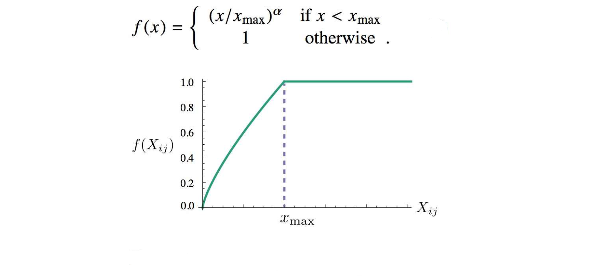
where

• f (0) = 0. That means, when \(X_{ij}=0\), the cost for word pair is not computed.
• f (x) should be non-decreasing so that rare co-occurrences are not overweighted.
• f (x) should be relatively small for large values of x, so that frequent co-occurrences are down-weighted (or not overweighted).

A large number of functions satisfy these properties, but one class of functions that is found to work well can be parameterized as follows:

Stochastic gradient or adaptive gradient updates (adagrad) can be used to optimize the model parameters. During each iteration, all the word and context vectors are updated.

According to Jeffrey Pennington, Richard Socher, and Christopher D. Manning (authors of GloVe), the model generates two sets of word vectors, \(W\) and \(\tilde{W}\) . When X is symmetric, \(W\) and \(\tilde{W}\) are equivalent and differ only as a result of their random initializations; the two sets of vectors should perform equivalently.

It has been shown that combining the results can help reduce overfitting and noise and generally improve results. Hence the authors of GloVe obtained the final word vectors by summing \(W\) and \(\tilde{W}\) to increase model performance and semantic analogy task.

“GloVe, is a new global log-bilinear regression model for the unsupervised learning of word representations that outperforms other models on word analogy, word similarity, and named entity recognition tasks.” (Pennington et. al, 2014)

GloVe is fast to train because only non-zero entries in the sparse co-occurrence matrix are used. GloVe can scale to huge corpora, performs well even with small corpus and small vectors. It has been found that the dimension of 300 is optimal for word vectors.

Evaluating Embeddings

There are different approaches for evaluating embeddings.

• Quantitative Evaluation: You could select some words and retrieve words similar to the selected word using semantic similarity search.
• Qualitative Evaluation: You can reduce the vector space into a three or two dimensional vector space, then visualize the words to see which words cluster together. PCA, t-SNE, UMAP. A good word embedding should have words that semantically related in the same cluster.

Transfer Learning and Embeddings

Pre-trained models can be used as they are or can be customized to a related new task through transfer learning. Transfer learning involves transferring knowledge learned by a pre-trained model from a large dataset for a specific task to a related new task. For example, you may training a fake news detector using a large data, then transfer the knowledge learned to a spam detection task.

Word embeddings can be pre-trained on large corpora of text data and then fine-tuned for specific NLP tasks, such as sentiment analysis and named entity recognition. Pre-trained word embeddings capture general language patterns and can be adapted to specific domains or tasks with additional training.

Whether you are re-using a model you already trained or a pre-trained model for a new task, transfer learning requires a model trained on a large and general dataset for a task to be customized to a related new task.

Transfer learning involves the following steps:

• Train your own model using a large and general dataset or get a pre-trained model.
• Retrain the pre-trained model on a new dataset to transfer knowledge from the pre-trained model to the new task.

There are couple of ways to retrain a pre-trained model:

1. If the data for the new task is small, you can retrain only the parameters of the last output layer and keep the rest of the parameters fixed by freezing the base layers of the network. The parameters of this output layer are trained from scratch.

2. If the data for the new task is large, you can retrain the parameters of all the layers in the neural network. In this case, retraining the learning algorithm starts with the weights that were previously learned, then updates the weights. Updating the weights of a pre-trained model by retraining the model is called fine-tuning, while the first training before retraining is known as pre-training.

Transfer learning has several advantages over classical machine learning:

• reduces training time by not build the model from scratch,
• improves performance,
• does not require large amount of data as knowledge learned from pre-trained models is leveraged.
• training a model from scratch can result to overfitting but transfer learning helps us to over this problem.

Note that another type of transfer learning is feature-based transfer learning where predictions generated from a pre-trained model are incorporated into new input used to train a completely new model.

It makes sense to transfer learning from a pre-trained model designed for task A to a new task B when:

• Task A and B have the same type of input such as text.
• Task A has a large dataset while task B has a small dataset
• Low dimensional features learned from task A are useful for task B.

Note that there is also multi-task learning where you train one neural network to do several tasks, with a better performance than training separate neural network for each task.