In this lesson, we will focus on linear models especially linear regression. Linear Regression is a model that captures or estimates the linear relationship between an output variable (y) and one or more input variables (\(x1\), \(x2\), etc). The input variable is also called an independent variable or a predictor. The output variable (\(y\)) is also called a dependent variable or an outcome.
The goal of linear regression: Linear regression has two major goals:
To find whether there is a significant statistical relationship between in the input variable (\(x\)) and output variable (\(y\)).
To estimate a linear model and use the estimated model to predict the output (\(y\)) when given the input (\(x\)).
In simple linear regression (with one independent variable), the model is:
\[
y = \beta_0 + \beta_1 x_1 + \epsilon
\]
\(y\): the dependent variable
\(x\): the independent variable
\(\beta_0\): the y-intercept (the value of \(y\) when \(x = 0\))
\(\beta_1\): the slope (how much \(y\) changes for a one-unit change in \(x\) or impact of \(x_1\) on \(y\).
\(\epsilon\): error term (the difference between the actual outcome and the predicted outcome)
In multiple linear regression (with more than one independent variable), the model extends to:
In multiple linear regression (with more than one independent variable), the model extends to:
\[
y = \beta_0 + \beta_1 x_1 + \beta_2 x_2
\] For simplicity, we will use a simple linear regression to explain the regression model. It is important to note that the “true” model or relationship is expressed as \(y = \beta_0 + \beta_1 x + \epsilon\) but in practice, we estimate the relation the relationship using an estimate of the model, \(\hat{y} = \beta_0 + \beta_1 x\).
Linear Regression Use Cases
Businesses could use linear regression to determine whether there is a strong linear relationship between advertising spending and sales revenue, and to measure the impact of their advertising budget on sales.
We could use linear regression to assess whether there is a statistically significant relationship between study hours and exam performance, and then predict exam scores based on the number of study hours.
Let’s simulate a linear regression to model the relationship between the outcome, \(\text{Exam Score}\), and the predictor, \(\text{Study Hour}\) The linear regression model for predicting exam scores based on study hours is:
\[
\text{Exam Score} = \beta_0 + \beta_1 \cdot \text{Study Hours} + \epsilon
\] This model can be estimated using: \[
\hat{\text{Exam Score}}= \beta_0 + \beta_1 \cdot \text{Study Hours}
\]
Exam Score and Study Hour Dataset: Let’s simulate some dataset for exam scores and study hours.
Code
import numpy as npimport pandas as pdimport matplotlib.pyplot as pltimport seaborn as sns# Set a random seed for reproducibilitynp.random.seed(123)# Simulate study hours (independent variable)study_hours = np.round(np.random.uniform(1, 10, 100), 1)# Simulate exam scores (dependent variable) with some noise# Assume a linear relationship: Exam Score = 50 + 5 * Study Hours + random noiseexam_scores =50+5* study_hours + np.random.normal(0, 10, 100)# Clip exam scores to be between 0 and 100exam_scores = np.clip(exam_scores, 0, 100)# Create a DataFramedata = pd.DataFrame({'study_hours': study_hours, 'exam_scores': exam_scores})# Display the first few rows of the datadata.head().style.format({'study_hours': '{:.2f}', 'exam_scores': '{:.2f}'})
study_hours
exam_scores
0
7.30
100.00
1
3.60
69.64
2
3.00
76.50
3
6.00
67.33
4
7.50
89.31
Given the study hours and exam scores data, we can fit a model (regression line) in the data. This regression line is an estimation of the relationship between Exam Scores and Study Hours and is expressed as: \[
\hat{\text{Exam Score}}= \beta_0 + \beta_1 \cdot \text{Study Hours}
\]\(\beta_0\) and \(\beta_1\) are the coefficients of the regression model and can be interpreted as follows:
\(\beta_0\) is the exam score that a student will have if they did not study (Study Hour = 0).
\(\beta_1\) is the impact or effect of study hours on exam scores.
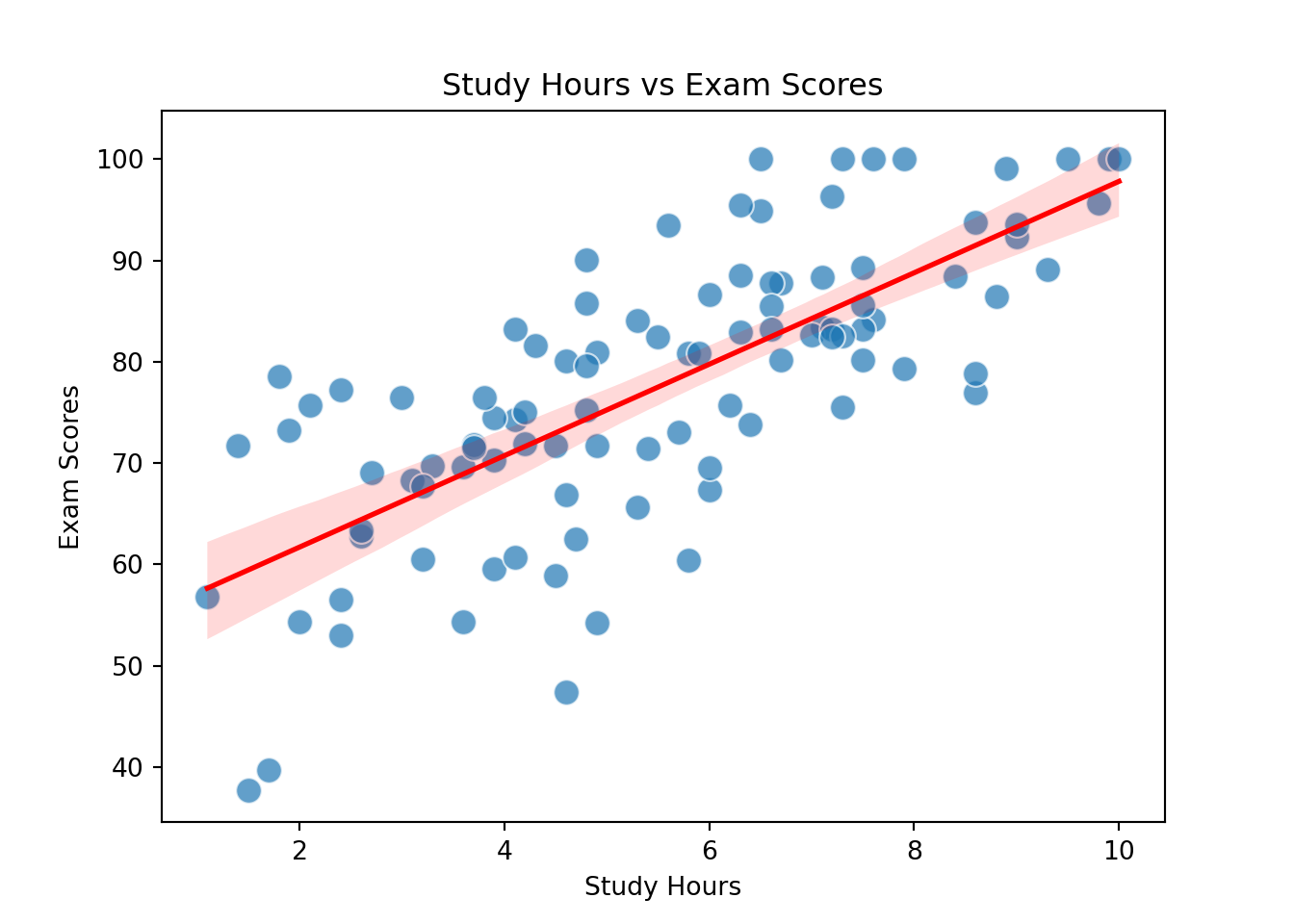
The line in the graph belows shows the relationship between Exam Scores and Study Hours
Code
# Create the plot using Seabornfig, ax = plt.subplots()ax = sns.scatterplot(x='study_hours', y='exam_scores', data=data, alpha=0.7, ax=ax, s=100)# Fit a linear regression line using Seaborn's regplot functionsns.regplot(x='study_hours', y='exam_scores', data=data, scatter=False, ax=ax, color='blue', line_kws={'color': 'red', 'lw': 2})# Set title and labels using the ax objectax.set_title('Study Hours vs Exam Scores')ax.set_xlabel('Study Hours')ax.set_ylabel('Exam Scores')# Show the plotplt.show()
How is the Regression Line Fitted in the Data?
The regression line representing the model can be fitted using a statistical technique called the Ordinary Least Squares (OLS) method. OLS is used to find the best-fitting line that minimizes the sum of squared errors (SSE). The goal of OLS is to find the values of \(\beta_0\) (intercept) and \(\beta_1\) (slope) that minimize the sum of squared errors.
Given a simple line regression line (model estimate):
\[
y = \beta_0 + \beta_1 x
\] The Sum of Squared Errors (SSE) measures the total deviation of the predicted values from the actual values. SSE is defined as:
\[
SSE = \sum_{i=1}^n (y_i - \hat{y}_i)^2
\]
Where:
\(y_i\) is the observed value,
\(\hat{y}_i\) is the predicted value of \(y_i\) based on the regression line.
The Sum of Squared Errors (SSE) expanded to include the coefficients is:
\[
SSE = \sum_{i=1}^n \left( y_i - (\beta_0 + \beta_1 x_i) \right)^2
\] The goal of OLS is to find the values of coefficients - \(\beta_0\) (intercept) and \(\beta_1\) (slope) - that minimize the sum of squared errors. This goal is achieved by finding the partial derivatives of SSE with respect to \(\beta_0\) and \(\beta_1\), setting the the partial derivatives to zero and solving for the coefficients, \(\beta_0\) and \(\beta_1\).
Partial Derivative with Respect to \(\beta_0\):
The partial derivative of SSE with respect to \(\beta_0\) is:
We can generate regression report that contains information about the linear relationship between study hours and exam scores:
Code
import statsmodels.api as sm# Prepare the independent variable (study_hours) and add a constant (intercept)X = sm.add_constant(data['study_hours']) # Adds a column of ones to X for the intercept# Dependent variable (exam_scores)y = data['exam_scores']# Fit the OLS regression modelmodel = sm.OLS(y, X).fit()# Display the summary tableprint(model.summary())
The two-tailed p-value, \(P > |t|\), is less than 0.01 for study hours, indicating that there is a statistically significant relationship between study hours and exam scores. This means that study hours significantly predict exam scores.
The coefficient of study hours, \(\beta_1 = 4.51\), indicates that for each additional hour of study, the exam scores are expected to increase by 4.51 points.
The intercept, \(\beta_0\) (const), is 52.67, which means that if a student does not study at all (study hours = 0), their expected exam score will be 52.67.
The p-value for the F-statistic is less than 0.01, suggesting that the model as a whole is statistically significant, i.e., the predictors (study hours) significantly explain the variation in exam scores. This p-value is particularly useful in multiple linear regression when there are several predictors.
The R-squared value is 0.539, meaning that study hours explain 53.9% of the variance in exam scores.
The simple regression model for predicting Exam Scores given Study Hours can then be formulated or estimated using the coefficient values of \(\beta_0\) and \(\beta_1\) as follows:
There are several assumptions of linear regression that need to be satisfied in order for us to generalize the regression results to the population represented by the training data used for modeling.
Here are the four key assumptions of linear regression:
Linearity: The relationship between the independent and dependent variables is linear, meaning changes in the independent variables result in proportional changes in the dependent variable. A scatter plot of the input and output variables should show linearity.
Normality of Errors: The residuals (errors) of the model should follow a normal distribution, with a mean of 0. Use a Q-Q plot (Quantile-Quantile plot), a histogram of the residuals, or the Shapiro-Wilk test to check if the residuals follow a normal distribution.
Constant Variance (Homoscedasticity): The variance of the residuals should remain constant across all levels of the independent variable(s). Plot residuals vs. predicted values. If the variance is constant, the spread of the residuals should be roughly the same across all levels of the predicted values.
Independence of Errors: The residuals should be independent of each other. This assumption is usually considered to be satisfied and is not usually tested.
Using Analytical Solutions vs Algorithms
The OLS (Ordinary Least Squares) approach for estimating a linear regression model is a statistical or analytical method with a greater focus on examining the impact of predictors on outcomes. This approach is popularly used by researchers to understand the effect of variables on an outcome of interest.
In machine learning, the focus is on finding a model that predicts the outcome of interest based on input data. While the statistical OLS approach can also estimate a model for predicting outcomes, machine learning typically uses algorithms like gradient descent instead of OLS. The regression model estimated through OLS and gradient descent would be similar, but there are advantages to using algorithms such as gradient descent over analytical methods like OLS, especially when dealing with large datasets or problems that are difficult to solve analytically.
For multiple regression, OLS requires that the matrix of independent variables (the design matrix) be non-singular, meaning it must be invertible. However, in some cases, the predictor matrix may not be invertible. This can occur when there is high multicollinearity among predictors (i.e., predictors are highly correlated with each other) or when there are more predictors than observations. In these situations, the matrix becomes singular, and OLS cannot compute a unique solution.
Gradient descent is especially beneficial when dealing with large datasets, high-dimensional data, or models that cannot be solved analytically with methods like OLS.
Gradient Descent
Gradient Descent is an iterative optimization algorithm used to estimate the parameters of a linear regression model by minimize the sum of squared errors using the gradient descent rule. The gradient descent starts with an initial guess for the coefficients and iteratively updates them in the direction that reduces the error.
The gradient descent update rule for estimating the coefficients \(b_j\) is given by: \[
b_j := b_j - \alpha \cdot \frac{\partial J}{\partial b_j}
\]
where:
\(\alpha\) is the learning rate,
\(\frac{\partial J}{\partial b_j}\) is the partial derivative of the cost function with respect to \(b_j\).
The cost function (Mean Squared Error) for linear regression is:
For \(b_1\): \[
\frac{\partial J(b_0, b_1)}{\partial b_1} = \frac{-2}{n} \sum_{i=1}^n (y_i - (b_0 + b_1 x_i)) x_i
\] Generally, the derivative of the cost function with respect to any coefficients \(b_j\) is given by:
\[
\frac{\partial J}{\partial b_j} = \frac{-2}{n} \sum_{i=1}^n (y_i - (b_0 + b_1 x_i)) x_{ij}
\] Where \(j\) = {0, 1, 2, 3,…k}. When \(j\) =0, x=1, and when \(j\)=1 corresponds to \(x_1\), etc.
Estimating a Linear Regression Model Using Gradient Descent
Code
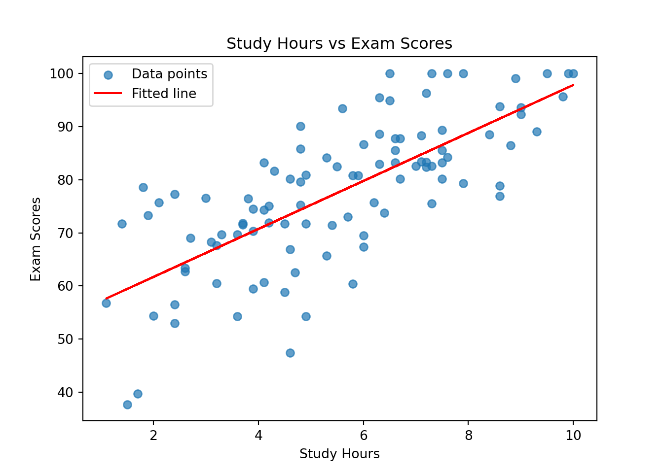
# Gradient Descent Functiondef gradient_descent(X, y, learning_rate=0.01, epochs=1000):# Number of data points m =len(y)# Initialize coefficients (b0 and b1)# using random values between 0 and 1. np.random.seed(1234) b0 = np.random.uniform(low=0, high=1) b1 = np.random.uniform(low=0, high=1)# Gradient Descent Loopfor _ inrange(epochs):# Predictions y_pred = b0 + b1 * X# Compute gradients b0_grad = (-2/m) * np.sum(y - y_pred) b1_grad = (-2/m) * np.sum((y - y_pred) * X)# Update coefficients b0 -= learning_rate * b0_grad b1 -= learning_rate * b1_gradreturn b0, b1# Prepare dataX = data['study_hours'].valuesy = data['exam_scores'].values# Run gradient descent to find b0, b1b0, b1 = gradient_descent(X, y, learning_rate=0.01, epochs=10000)# Print the learned coefficientsprint(f"Intercept (b0): {b0:.2f}", "\n",f"Slope (b1): {b1:.2f}")
Intercept (b0): 52.67
 Slope (b1): 4.51
Code
# Plot the data and the fitted lineplt.scatter(X, y, alpha=0.7, label="Data points")plt.plot(X, b0 + b1 * X, color='red', label="Fitted line")plt.title("Study Hours vs Exam Scores")plt.xlabel("Study Hours")plt.ylabel("Exam Scores")plt.legend()plt.show()
There are different types of gradient descent:
Batch Gradient Descent: the entire dataset is used to compute the gradient and update the model parameters in each iteration.
Stochastic Gradient Descent (SGD): a single random data point (record) is used to compute the gradient and update the model parameters in each iteration.
Mini-Batch Gradient Descent: the dataset is divided into small or mini batches, and a random mini-batch of the training data is used to compute the gradient and update the model parameters in each iteration.
We wrote this gradient descent (batch gradient descent) optimization algorithm above from scratch to show how the gradient descent algorithm works. This hands-on implementation helps us understand the mechanics of updating coefficients iteratively using the cost function, Mean Squared Error. However, in practice, you can use machine learning frameworks such as scikit-learn, which contains more efficient and optimized estimators for regression problems, including those that implement gradient descent.
Regressions in Scikit-learn
Scikit-learn is a popular and widely used machine learning library in Python. It provides tools and algorithms for classification, regression, clustering, dimensionality reduction, model selection, and preprocessing. For the rest of this lesson, we will focus on regression models. Classification and clustering models will be covered in subsequent lessons.We will use the study hours and exam scores dataset to illustrate how to implement regression models in sklearn.
Linear Regression in Scikit-learn
A linear regression model is implemented in sklearn as follows. This examples shows the packages needed, how to prepare in input and output data, split the data, initialize the model, fit the model, make predictions, and evaluate the model’s performance on the test and training datasets.
Code
import numpy as npfrom sklearn.linear_model import LinearRegressionfrom sklearn.model_selection import train_test_splitfrom sklearn.metrics import mean_squared_error# dataX = data['study_hours'].values.reshape(-1, 1) y = data['exam_scores'].values# Split data into training and test setsX_train, X_test, y_train, y_test = train_test_split(X, y, test_size=0.2, random_state=42)# Initialize and train the modelmodel = LinearRegression()model.fit(X_train, y_train);# Make predictionsy_pred = model.predict(X_test)# Evaluate the modelmse = mean_squared_error(y_test, y_pred)print(f"Mean Squared Error: {mse}", "\n",f"Coefficient (b1): {model.coef_[0]}", "\n",f"Intercept (b0): {model.intercept_}")
Mean Squared Error: 73.57852774601953
 Coefficient (b1): 4.6938248069933035
 Intercept (b0): 51.38763147736775
Gradient Descent for Regression Tasks in Scikit-learn
Code
import numpy as npimport pandas as pdfrom sklearn.linear_model import SGDRegressorfrom sklearn.model_selection import train_test_splitfrom sklearn.metrics import mean_squared_error# DataX = data['study_hours'].values.reshape(-1, 1) # Independent variable (study hours)y = data['exam_scores'].values # Dependent variable (exam scores)# Split the data into training and testing setsX_train, X_test, y_train, y_test = train_test_split(X, y, test_size=0.2, random_state=42)# Initialize the SGDRegressor (with gradient descent optimization)model = SGDRegressor(max_iter=1000, tol=1e-6, eta0=0.01) # Learning rate = 0.01# Train the model using the training datamodel.fit(X_train, y_train);# Make predictions using the test datay_pred = model.predict(X_test)# Evaluate the modelmse = mean_squared_error(y_test, y_pred)print(f"Mean Squared Error: {mse}\n"f"Coefficient (b1): {model.coef_[0]}\n"f"Intercept (b0): {model.intercept_}")
Mean Squared Error: 89.96121836819495
Coefficient (b1): 5.635108625357887
Intercept (b0): [45.13423073]
Random Forest for Regression Tasks in Scikit-learn
Note that random forest can be used to solve regression problems but random forest is a non-linear model suitable for a dataset where the relationship in the data is assumed to be non-linear.
Code
import numpy as npimport pandas as pdfrom sklearn.ensemble import RandomForestRegressorfrom sklearn.model_selection import train_test_splitfrom sklearn.metrics import mean_squared_error# Independent variable (study_hours) and dependent variable (exam_scores)X = data['study_hours'].values.reshape(-1, 1) # Reshape for sklearn modely = data['exam_scores'].values# Split data into training and testing sets (80% training, 20% testing)X_train, X_test, y_train, y_test = train_test_split(X, y, test_size=0.2, random_state=42)# Initialize the RandomForestRegressormodel = RandomForestRegressor(n_estimators=100, random_state=42)# Train the model with the training datamodel.fit(X_train, y_train);# Make predictions with the test datay_pred = model.predict(X_test)# Calculate Mean Squared Errormse = mean_squared_error(y_test, y_pred)# Print the resultsprint(f"Mean Squared Error: {mse}\n"f"Feature Importances: {model.feature_importances_}\n"f"Predictions: {y_pred[:5]}") # Show first 5 predictions
In this lesson, we focused on the linear regression model, a foundational machine learning model. Linear regression, one of the simplest and most commonly used models, aims to model the relationship between a dependent variable (like exam scores) and one or more independent variables (like study hours). There are two types of linear regression models: simple linear regression and multiple linear regression.
Both capture the linear relationship in the data and are used to predict the dependent variable based on the inputs. Linear regression involves estimating coefficients that minimize the sum of squared errors, typically using the Ordinary Least Squares (OLS) approach. For real-world applications, such as predicting exam scores from study hours, this technique provides valuable insights into how variables are correlated and helps in making predictions.
The use of regression analysis extends beyond linear models. Machine learning algorithms such as Gradient Descent and Random Forest regression are also valuable tools for more complex datasets. Gradient descent is an optimization technique used to minimize the cost function iteratively and is particularly useful for large datasets where analytical methods like OLS are inefficient.
On the other hand, Random Forest regression offers a non-linear approach suitable for datasets where relationships between variables are non-linear, making it a powerful tool for regression tasks with high-dimensional or non-linear data. These models are widely used in practical machine learning workflows and can be easily implemented with libraries such as Scikit-learn, which provides efficient algorithms for training and evaluation.
 The goal of linear regression: Linear regression has two major goals: