Lessonn 19: Encoder Decoder Models

Encoder Decoder Models

Encoder decoder models, also called sequence-to-sequence models are models that take an input sequence and generates an output sequence that is of a different length than the input sequence, without any one-to-one alignment between the input sequence and output sequence words.

Encoder decoder models are very useful for NLP tasks such as machine translation. These models are also used for other tasks such as text summarization and question answering.

The encoder decoder network architecture have two components, the encoder and the decoder. The encoder and decoder can be any sequence architecture such as RNNs, LSTMs, or transformers.

A simple Encoder Decoder Architecture with RNNs

Below is a simple encoder decoder architecture with RNNs:

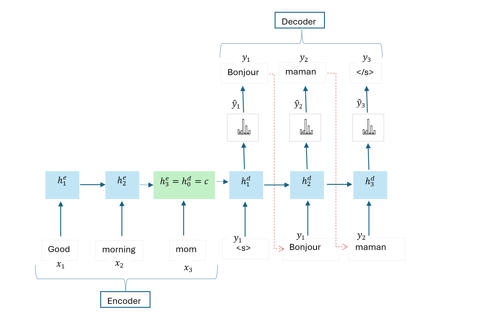
1. The encoder network takes an input sequence and transforms it into a fixed length latent representation or context vector.

2. The decoder network uses the last hidden state of the encoder \(c = h_0^d\) as its initial hidden state and the start-of-sequence token \(<s>\) to generate an output sequence of words until the end-of-sequence token \(</s>\) is reached.

Training an Encoder Decoder Model

During training, a training sample consists of an input sequence of token \(x\) and the corresponding output sequence of ground truth target tokens \(y\) to be generated. Hence supervised learning is used for training the model. Note that the input sequence \(x = {x_1, x_2, ... x_n}\) is used as input into the encoder network while the output sequence of ground truth target tokens \(y = {y_1, y_2, ... y_m}\) is used as input into the decoder network.

During training, the forward pass of a simple encoder decoder model involves using the encoder network to encode the input sequence into a hidden representation (context vector). At any time step t, the hidden state of the encoder network takes the previous hidden state and the current input sequence token:

\[ h_t^e = g(h_{t-1}^e, x_t) \] The last hidden representation of the encoder network \(c = h_0^d\) and the start-of-sequence \(<s>\) are used to initialize the decoder network. At any time step t, the hidden state of the decoder network is computed using the previous hidden state \(h_{t-1}^d\) and the previous target output \(y_{t-1}\):

\[ h_t^d = g(h_{t-1}^d, y_{t-1}) \]

The decoder network uses teacher forcing during the forward pass where the embedding of the actual previous output \(y_{t-1}\) instead of the predicted output (with highest probability) is used as input into the next time step.

During backpropagation, the loss at each time step is computed using the softmax loss with the training objective of maximizing the probability of the correct output token at that time step.

\[\begin{align} l_t(\theta)_{max} &= P(y_{t, correct}|\text{context}) \\ l_t(\theta)_{min} &= - \log \hat{y}_{t, correct} \end{align}\]

The loss for the entire sentence is the sum (or average) of the individual losses at different time steps:

\[\begin{align} L(\theta) &= \sum_{t=1}^T l_t(\theta) \\ &= - \sum_{t=1}^T \log \hat{y}_{t,correct} \end{align}\]

Once the loss \(L\) is computed, gradients of the loss with respect to all model parameters (both encoder and decoder) are computed using backpropagation through time (BPTT).

These gradients are then used to update the parameters of the model using an optimization algorithm (e.g., SGD, Adam) to minimize the loss.

Inference with a Trained Encoder Decoder Model

At inference time in a sequence-to-sequence model, the process is different from training because the model is used to generate output sequences without the ground truth target tokens provided as inputs to the decoder

During inference:

• the input sequence is fed into the encoder network of the trained sequence-to-sequence model to encode the sequence into a final hidden state (context vector).
• the decoder uses the final hidden state of the encoder as its initial hidden state. The start-of-sequence is also used as the initial input into the decoder.
• In a simple inference where greedy decoding is used, at each time step t, the model generates a probability distribution over the target words using the softmax function; \(softmax(W_yh_t^d)\) where \(W_h\) is a weight matrix for the weights associated with the output layer and \(h_t^d\) is the hidden layer at time step t.
• The predicted output token with the highest probability is then selected using the argmax of the probability distribution.
• The predicted output token then become the input to the decode for the next time step.

Limitation of the Simple Encoder Decoder with RNN

One limitation of the simple encoder decoder with RNN is that the context information captured through the encoder and used to initialize the decode may diminish as the decoder progresses, hence the decoder may not be able to capture long-term dependencies.

A More Complex Encoder Decoder Architecture with RNNs

To solve this problem of long-term dependencies, a more complex encoder decoder architecture with RNNs can be used, where the context captured by the encoder is passed directly to each of the decoder’s hidden state at any time step t, as shown below:

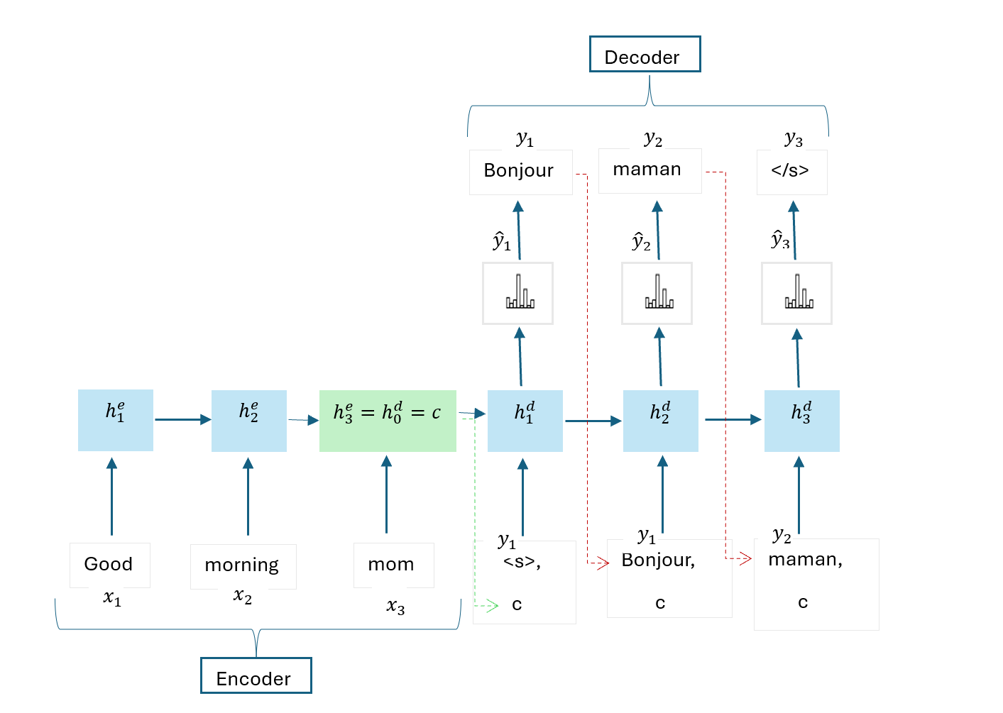
This architecture is very similar to the simple encoder decoder with RNN except that the decoder’s hidden state for the complex sequence-to-sequence model at any time step t is computed as:

\[ h_t^d = g(h_{t-1}^d, y_{t-1}, c) \] where:

• \(c\) is the final hidden state of the encoder, \(h_n^e = h_0^d\)
• \(h_{t-1}^d\) is the previous hidden state of the decoder
• \(y_{t-1}\) is the previous ground truth target output token used during training if teacher forcing is implemented. At inference time, \(y_{t-1}\) is replaced with the predicted previous output token \(\hat{y}_{t-1}\) having the highest probability.