Simple Neural Language Models
Simple Neural Language Models
Language models predict the next word given a sequence of context words. Neural language models are language models based on neural networks. Examples of neural language models include feed forward neural language models and language models with transformers architecture, which power modern NLP applications. Simple neural language models in this lesson refer to simple feed forward neural language models.
Why neural language models?
N-gram language models can result to inaccurate predictions due to sparsity issues, zero counts, and zero probabilities if unseen input context did not appear in the training data. Neural language models generalize well to similar context when trained with word embeddings, resulting to more accurate predictions.
If word embedding are used to train a neural language model, suppose the training corpus for learning the embeddings had a sequence of words my cat likes tuna, then neural networks trained with word embeddings can use the similarity of “cat” and “dog” embeddings to generalize and predict “tuna” as the next word in the sentence, my dog likes____.
Training an n-gram language model is computationally expensive if the n-gram is large (or if the sequence of context words is too long). Neural language models have advantages over n-gram models because neural models can handle longer context histories efficiently by pooling word vectors of context words.
Moreover, there is no need to store all n-gram counts and probabilities with neural language models, hence neural networks allow efficient storage.
Nevertheless, neural networks with many layers and nodes can be complex, less interpretable and slow to train, so n-grams are still good for smaller tasks.
A simple feed forward neural language model architecture
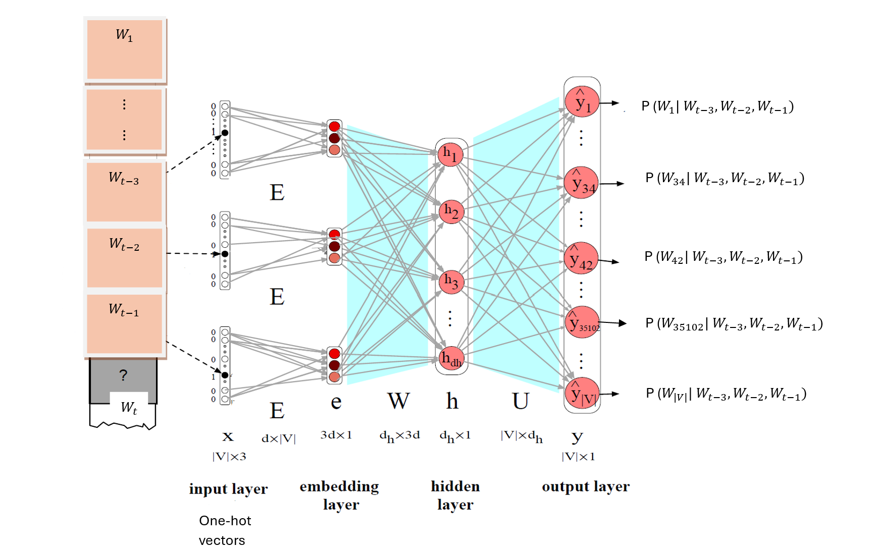
A simple feed forward neural network consists of:
- an input layer: one-hot vectors of context words,
- an embedding layer: concatenated or pooled context word embeddings
- a hidden layer: hidden representation of context words, and
- an output layer: softmax layer with the probabilities of vocabulary words.
Self-supervised learning
Self-supervised learning is used to train neural language models, where the target for the model’s prediction task is derived directly from the training corpus allowing the model to learn useful representations of the language without requiring manually labeled data. This self-supervised learning approach has proven to be effective in training language models on large amounts of unlabeled text data.
How are simple feedforward neural language networks trained?
Just like any other neural network, training a neural language network involves a forward pass, computing loss, backpropagation, updating weights.
Forward Pass: During the forward pass, the input one-hot vectors of context words are fed into the neural network. The one-hot context vectors \(x\) are then transformed by a shared embedding matrix \(E\) into context word embeddings. The context word embeddings are concatenated into an embedding layer, \[e=[Ex_{t-3};Ex_{t-2};Ex_{t-1}]\] The columns of the embedding matrix are embedding vectors of vocabulary words in the corpus. The embedding matrix could be used as a look up table, in practice.
The concatenated context word embeddings are transformed by the weight matrix, \(W\) into weighted sums of the embedding vector entries. An activation function is then applied element-wise to the weighted sums to obtain outputs represented as the hidden layer, \[h = \sigma(We + b) \] The hidden layer is further transformed by another weighted matrix \(U\) into weighted sums of the hidden vector entries. The softmax function is applied to the weighted sums to generate the probability of vocabulary word given the context words,
\[\begin{align} \hat{y} &= softmax(z) \\ &= \frac{e^{z_i}}{\sum^{|V|}_{j=1}e^{z_j}} \end{align}\]
where \[ z = Uh \] Compute Loss: Once the output layer produces a prediction, the difference between the predicted output and the actual output (the ground truth) is computed using a loss function. The loss function quantifies how far off the prediction is from the actual target. The loss of the softmax function maximizes the probability of the correct next word given the context:
\[\begin{align} L(\theta)_{max} &= P(y_c|\text{context words}) \\ L(\theta)_{min} &= - \sum^{|V|}_{j=1} y_j \log \hat{y}_j \\ &= - y_c \log \hat{y}_c \\ &= - \log \hat{y}_c \end{align}\]
\(\mathbf{y}\) is a one-hot encoded vector where its entries are represented as \(y_i\), with each entry corresponding to a class. The true class has a value of 1, and all other classes are represented as 0. That is, \(y_i = y_c = 1\) for the correct class and 0 for all others. \(i\) is the index of the entries in the one-hot vector, while \(|V|\) is the vocabulary size (total number of classes or the size of the one-hot vector).
Since \(\mathbf{y}\) is a one-hot vector with entry \(y_i = 1\) for the correct class and \(y_i = 0\) for other classes, the sum reduces to a single term, which is the term at the index of the correct class. Hence, the loss simplifies to:
\[ L = - \log(\hat{y}_{\text{c}}) \]
Backward Pass (Backpropagation): In this step, the algorithm works backward through the network, calculating the gradient of the loss function with respect to each weight and bias in the network. This gradient represents the direction and magnitude of change needed to reduce the loss. Backpropagation computes these gradients efficiently using the chain rule of calculus.
The gradient of the softmax loss function with respect to the weights in the softmax layer can be written as:
\[ \frac{\partial J (\theta)}{\partial \theta_j} = \frac{\partial J (\theta)}{\partial \hat{y}_c} \cdot \frac{\partial \hat{y}_c}{\partial z_c} \cdot \frac{\partial z_c}{\partial \theta_j} \] where:
\[\begin{align} J(\theta) &= - y_c\log \hat{y}_c \\ \hat{y}_c &= \frac{exp(z_c)}{\sum_{i=1}^{|V|} exp(z_i)} \\ z_i &= \sum_{j=1}^{k} \theta_{ij} \cdot h_j = W \cdot h \end{align}\]
- \(z_i\) is the pre-activation for class \(i\),
- \(k\) is the number of input features including the bias term,
- \(h_j\) is the \(j\)-th hidden input feature,
- \(\theta_{ij}\) is the weight corresponding to the \(j\)-th hidden input feature for class \(i\)
- |V| is the size of the vocabulary in the corpus.
Hence
\[\begin{align} \frac{\partial J (\theta)}{\partial \theta_{ij}} &= -y_c(1 - \hat{y}_c) \cdot h_j \\ &= -(y_c - \hat{y}_c) \cdot h_j \\ &= -(1 - \hat{y}_c) \cdot h_j \end{align}\]
Note that in each stochastic gradient descent iteration, only the error for the correct class \(y_c - \hat{y}\) is used to update the weights.
This derivative of the softmax loss function above is computed only with respect to the weights in the last layer. However, the derivative needs to be computed with respect to all weights in the network. For weights in the hidden or earlier layers, backward differentiation can be used to compute the derivative of the loss function with respect to those weights. Each node in a layer is a function whose derivatives with respect to the weights in that node can be computed and used in backward differentiation.
Update Weights: Finally, the weights and biases of the network are adjusted in the opposite direction of the gradient, using a technique called gradient descent or one of its variants (such as stochastic gradient descent, Adam, RMSprop, etc.). This update step aims to minimize the loss function, effectively improving the model’s performance over time.
The stochastic gradient descent rule used to update the weights is as follows:
\[ \theta := \theta - \alpha \frac{\partial J(\theta)}{\partial \theta} \]
Challenges with Neural Language Models
Some challenges with neural language models includes the fact that the sliding fixed context window could be too small and increasing it’s size also increases the size of the embedding matrix, \(W\) since embeddings need to be concatenated and multiplied to W.
Also, using a fixed-size window can be problematic because if a neural network is trained with a fixed window, then the size of the input sequence must be consistent with the size of the fixed window used for training.
Fixed-size window require input sequences to be of a consistent length. However, natural language often involves variable-length sequences, such as sentences or documents of different lengths. Requiring all inputs to conform to the fixed window size introduces the need for padding (adding dummy values) or truncation (cutting off parts of the sequence), which can lead to information loss or inefficiency.
The inflexibility of feed forward neural language models with variable-length sequences can be handled naturally with RNNs without requiring padding or truncation. RNNs process input sequences one element at a time, updating their internal states recursively, which allows them to accommodate inputs of different lengths.