Lesson 16: Neural Networks for Text Classification
Neural Networks for Text Classification
In this lesson we will focus on feed forward neural networks for text classification use cases such as spam classification and sentiment analysis. Using neural networks with word embeddings is much better than using n-gram language models. This is because word embeddings represents words that are similar in meaning using a similar vector distribution.
Neural Networks for Binary Classification
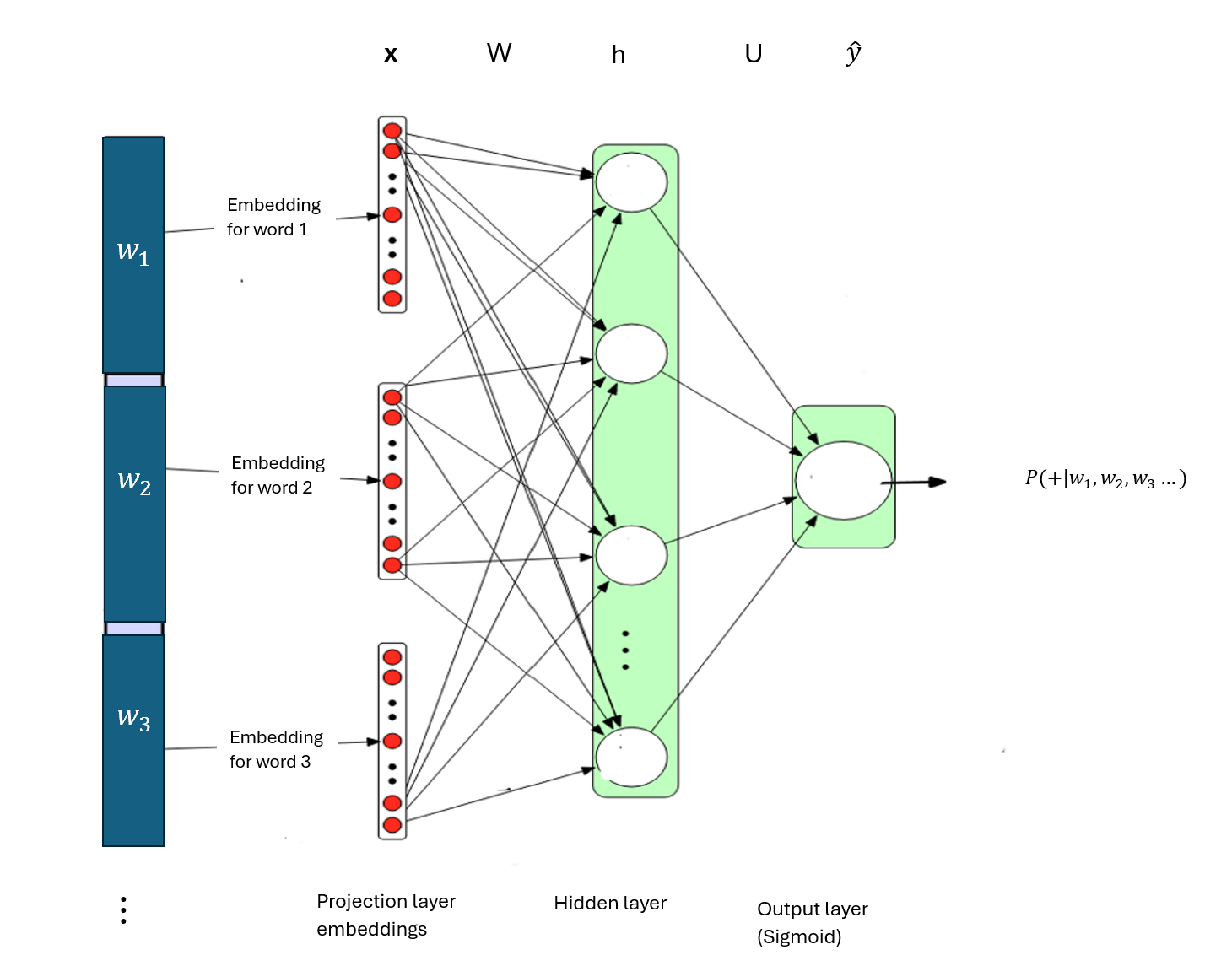
Neural networks can be used for binary classification of text. For example: neural networks can be used for a sentiment analysis task to predict whether the sentiment in a document or piece of text is positive or negative.Below is a simple feed forward neural networks for binary classification of text.
where
- \(x = [e(w_1), e(w_2), \ldots, e(w_n)]\)
- \(h = \sigma(W.x)\)
- \(z = U.h\)
- \(\hat{y} = \sigma(z)\)
The input layer consists of word embeddings of words in a document. The word embeddings in each document are stacked or concatenated in the input layer to produce an input vector, \(x\) representing the document. If the length of each embedding is \(d_e\), and there are \(n\) words in the document, then the length of document vector \(x\) is \(d_x = n*d_e\). Hence the dimension of the input document vector is \(d_x\)x1.
This approach of stacking word embeddings to obtain a document vector assumes that all documents have the same number of words. However, this assumption is unrealistic. In practice, a fixed length for the document vector is defined, and padding with zeros or truncation is used to adjust any document vector with length shorter or longer than the defined length. Other approaches such as element-wise averaging or element-wise max of word embeddings is used to obtain a document vector with a fixed length.
The hidden layer consists of nodes that use the weight matrix \(W\) to transform the document vector \(x\) into a weighted scores, which are further transformed by the sigmoid activation function.
\[h = \sigma(W.x)\]
Note that the bias term be could be explicitly added so that \(h = \sigma(W.x+b)\) where \(x = x_1, x_2, \ldots, x_n\) but for this lesson, we will use \(h = \sigma(W.x)\) where \(x = x_0, x_1, x_2, \ldots, x_n\).
- The length of the hidden vector \(h\) is \(d_h=\) number of nodes in the hidden layer. Hence the dimension of \(h\) is \(d_h\)x1.
- The length of the input vector \(x\) is \(d_x\), hence the dimension of \(x\) is \(d_x\)x1.
- The dimension of the weight matrix \(W\) is \(d_h\)x\(d_x\).
The output layer transforms the hidden vector \(h\) using a weight matrix \(U\) into a single score \(z\) through a dot product multiplication. \[z = U.h\] \(U\) is a 1x\(d_h\) matrix while \(h\) is a \(d_h\)x1 vector. Note that row and column vectors are a special type of matrix with dimensions, 1xk or kx1 respectively. Hence, though \(U\) is a row vector in the situation of a binary classification, we can still call it a matrix as weights are conventionally called matrix while the inputs and outputs are special matrix (column vectors) conventionally called vectors.
The weighted score, z is then passed into the sigmoid function to generate the probability of the sentiment being positive given the document.
\[\begin{align} \hat{y} &= \sigma(z) \\ &= P(+|\text{the sequence of words in the document}) \\ &= \frac{1}{1 + e^{-z}} \end{align}\]
Training a neural network for binary classification
Stochastic gradient descent optimization can be used to train a neural network for binary classification. A single sample (or document) is used to train the network model during each iteration. During each iteration, the feed forward network is used to estimate the probability of classifying the sample into class one and back propagation is used to update the weights of the neural network.
The objective of the neural network for binary classification
For a single training example using a SGD, the training objective of neural network for binary classification is to maximize the probability of the true labels given the input document. That means,
- if the actual label is 1 (or positive), the objective is to maximize \(P(y=1|x)\).
- if the actual label is 0 (or negative), the objective is to maximize \(1-P(y=1|x)\).
Note that \(P(y=0|x) = 1-P(y=1|x)\).
The two objectives above can be mathematically summarized using a piecewise function for a single training example as follows:
\[ L(\theta)_{max} = \begin{cases} P(y=1|x) & \text{if } y = 1 \\ 1 - P(y=1|x) & \text{if } y = 0 \end{cases} \] The piecewise function can be written as a single mathematical statement for a single training example as follows:
\[ L(\theta)_{max} = P(y{_i}=1|x)^{y_i} (1-P(y{_i}=1|x))^{(1-y_i)} \] For simplicity and convenience, let’s drop the “i” representing the ith training example in the formulas.
For a binary classification
\[P(y=1|x) = \sigma(z)\]
Hence
\[L(\theta)_{max} = \sigma(z)^{y} (1-\sigma(z))^{1-y}\]
Maximizing the likelihood of \(\theta\) is the same as minimizing the negative likelihood of \(\theta\).
\[\begin{align} L(\theta)_{min} &= - L(\theta)_{max} \\ &=- \sigma(z)^{y} (1-\sigma(z))^{1-y} \end{align}\]
Since it is mathematically easier to work with log likelihood in addition to the fact that likelihood and log likelihood are monotonically increasing functions, we can write the objective function (aka cross-entropy loss) as follows:
\[\begin{align} L(\theta)_{min} &= - \log \sigma(z)^{y} (1-\sigma(z))^{y}) \\ &= - [y\log\sigma(z) + (1-y)\log (1-\sigma(z))] \end{align}\]
Updating the weights of the neural network for binary classification
Remember that for a logistic regression:
- Input feature vector: \(x = (x_1, x_2, ..., x_k)\).
- Predicted probability: \(\hat{y} = \sigma(z) = \frac{1}{1 + e^{-z}}\), where \(z = \theta^Tx = \sum_{j=1}^k \theta_jx_j\)
- True label: \(y\).
- Loss for a single training example: \[J(\theta) = L(\theta) = - [y\log \hat{y} + (1-y)\log (1-\hat{y})]\]
The gradient of the logistic regression loss function for a single training example is derived as follows.
From the chain rule of differentiation: \[\frac{\partial J(\theta)}{\partial \theta_j} = \frac{dJ(\theta)}{d\hat{y}} \cdot \frac{d\hat{y}}{d\theta_j}\] Where
\[\frac{dJ(\theta)}{d\hat{y}} = -\left(\frac{y}{\hat{y}} - \frac{1-y}{1-\hat{y}}\right) \] and
\[\begin{align} \frac{\partial \hat{y}}{\partial \theta_j} &= \frac{d\hat{y}}{\partial z} \cdot \frac{\partial z}{\partial \theta_j} \\ &= \frac{\partial}{\partial z} (\frac{1}{1 + e^{-z}}) \cdot \frac{\partial z}{\partial \theta_j} \end{align}\]
Note that we can find \(\frac{\partial \hat{y}}{\partial z}\) using the quotient rule of differentiation and \(\frac{\partial z}{\partial \theta_j} = x_j\).
So
\[\begin{align} \frac{\partial \hat{y}}{\partial \theta_j} &= \frac{d}{\partial z} (\frac{1}{1 + e^{-z}}) \frac{\partial z}{d\theta_j} \\ &= \frac{0 \cdot (1 + e^{-z}) - 1 \cdot (-e^{-z})}{(1 + e^{-z})^2}\cdot x_j \\ &= \frac{e^{-z}}{(1 + e^{-z})^2}\cdot x_j \\ &= \frac{1}{1 + e^{-z}} \cdot \frac{e^{-z}}{1 + e^{-z}}\cdot x_j \\ &= \frac{1}{1 + e^{-z}} \cdot \frac{1 + e^{-z} - 1}{1 + e^{-z}}\cdot x_j \\ &= \hat{y} \cdot (1 - \hat{y})\cdot x_j \end{align}\]
Finally
\[\begin{align} \frac{\partial J(\theta)}{\partial \theta_j} &= -\left(\frac{y}{\hat{y}} - \frac{1-y}{1-\hat{y}}\right) \cdot \hat{y} \cdot (1 - \hat{y})\cdot x_j \\ &= (\hat{y} - y) \cdot x_j \end{align}\]
For training the network, we need the derivative of the loss with respect to each weight in every layer of the network. The derivative of the logistic regression cost function above only updates the weight in the output layer. To update weights in the hidden layer of a deep neural network, computation graphs with backward differentiation can be used to find derivatives with respect to weights in early layers of a deep network.
Neural Networks for Multiclass Classification
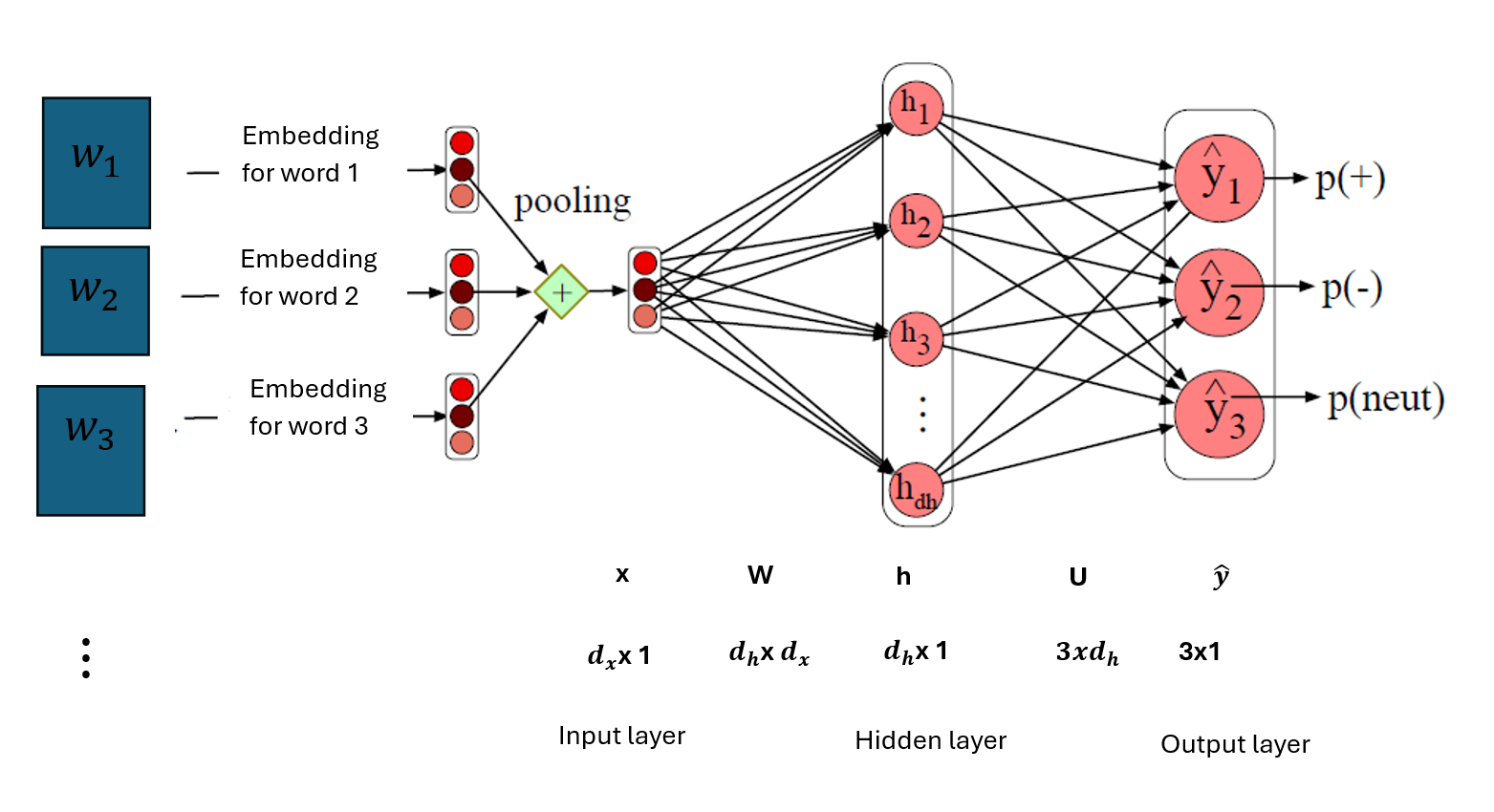
Neural networks can be used for multiclass classification of text. For example, a neural network can be used for a sentiment analysis of text documents where there are multiple classes such as positive, negative and neutral. A neural networks for a multiclass classification is an adjustment of the neural network for binary classification of text where the sigmoid function in the output layer is replaced with a softmax function.
The input layer applies a pooling function to the embeddings of all words in the document. The pooling function basically could be an element-wise addition or element-wise average of the word embedding in a document.
where
- \(x = \text{mean}(e(w_1), e(w_2), \ldots, e(w_n))\)
- \(h = \sigma(Wx)\)
- \(z = U.h\)
- \(\hat{y} = softmax(z)\)
Training the neural network for multiclass classification
The training objective of the neural network for multiclass classification is to maximize the probability of the correct class, \(c\).
\[\begin{align} L(\theta)_{max} &= P(y_c|document) \\ &= P(y_c|w_1, w_2, w_3, ..., w_n) \\ &= softmax(z_c) \\ &= \frac{exp(z_c)}{\sum_{j=1}^{C} exp(z_j)} \\ &= \hat{y_c} \end{align}\]
The probability of the correct class, \(P(y_c|document)\) can be written in various ways. If there are \(C\) possible classes \(y = \{y_1, y_2, y_3, ..., y_C\}\), then y can be a one-hot encoded such that \(y_i=1\) for the correct class and 0 for all other classes. For example, if the correct class is \(y_2\) then, y can be a one-hot vector represented as \(y=[0, 1, 0, ...,0]^T\).
Supposed y is one hot encoded, where \(y_i\) is 1 for the correct class \(y_c\) and 0 for all other classes, we can write the probability of the true class as follows:
\[\begin{align} P(y_c|document) &= \prod^C_{i=1} P(y_i|w_1, w_2, w_3, ..., w_n)^{y_i} \\ \end{align}\]
Therefore, the cost function for a multiclass classification with a softmax output is as follows:
\[\begin{align} J(\theta)_{max} &= P(y_c|document) \\ &= \prod^C_{i=1} P_i(y_i|w_1, w_2, w_3, ..., w_n)^{y_i} \\ &= \prod^C_{i=1} \hat{y_i} ^{y_i} \end{align}\]
where i represents the \(ith\) class.
The objective function can also be formulated as a minimization of the negative log likelihood of the softmax function.
\[\begin{align} L(\theta)_{min} &= - \log \prod^C_{i=1} \hat{y_i} ^{y_i} \\ &= - \sum^C_{i=1} \log \hat{y}_i ^{y_i} \\ &= - \sum^C_{i=1} {y_i} \log \hat{y}_i \\ &= - y_c \log \hat{y}_c \\ &= - \log \hat{y_c} \end{align}\]
where \(c\) is the correct class and \(C\) the number of possible classes.
Training a neural network for multiclass classification
The stochastic gradient descent rule can be used to learn the parameters of a neural network:
The gradient of the soft max cost function with respect to the weights in the output layer is derived using the chain rule as follows:
\[ \frac{\partial J (\theta)}{\partial \theta_{ij}} = \frac{\partial J (\theta)}{\partial \hat{y}_c} \cdot \frac{\partial \hat{y}_c}{\partial z_c} \cdot \frac{\partial z_c}{\partial \theta_{ij}} \] Let’s consider a case of a softmax regression, a neural network for multiclass classification with an input and output layer where the output layer has multiple nodes corresponding to various possible classes.
A softmax regression is an extension of a binary logistic regression where the output is the probability of multiple classes instead of the probability of one class.
We can derive the gradient of the cost function using the chain rule because the cost function is a composite function in the form f (x) = u(v(w(x))):
\[ J(\theta) = - y_c\log \hat{y}_c\] \[ \hat{y}_c = \frac{exp(z_c)}{\sum_{i=1}^{C} exp(z_i)}\]
\[ z_i = \sum_{j=1}^{k} \theta_{ij} \cdot x_j = W \cdot x \]
where:
- \(z_i\) is the pre-activation for class \(i\),
- \(k\) is the total number of features including the bias term,
- \(x_j\) is the \(j\)-th input feature,
- \(\theta_{ij}\) is the weight corresponding to the \(j\)-th input feature for class \(i\).
- \(C\) is the possible number of classes in the target.
- Compute the derivative of the loss with respect to the predicted probability of the correct class:
\[ \frac{\partial J(\theta)}{\partial \hat{y}_c} = -\frac{y_c}{\hat{y}_c} \]
- Compute the derivative of the predicted probability of the correct class with respect to the pre-activation of the correct class:
\[ \frac{\partial \hat{y}_c}{\partial z_c} = \hat{y}_c \times (1 - \hat{y}_c) \]
- Compute the derivative of the pre-activation of the correct class with respect to the parameter \(\theta_j\).
\[ \frac{\partial z_c}{\partial \theta_{ij}} = x_j \] 4. Combine the derivatives using the chain rule:
\[ \frac{\partial J (\theta)}{\partial \theta_{ji}} = -\frac{y_c}{\hat{y}_c} \times \hat{y}_c \times (1 - \hat{y}_c) \times x_j \]
The derivative of the softmax regression above only updates the weight in the output layer. For a deep neural network with hidden layers, a computation graph and backward differentiation can be used to update weights in the hidden layers.
Each node in a neural network is a function. With backward differentiation, we find the derivatives of the functions in the nodes and use these derivatives to compute derivative of the loss with respect to the weights in the early or hidden layers.
Some good practices for training neural networks include:
- initializing weights with small random values.
- standardizing the input to have a mean of zero and variance of 1. That is, transform the input using: \(\text{standardized}(x) = \frac{x - \mu}{\sigma}\)
- the random dropout of nodes and their connections during training can prevent overfitting.
- the tuning of hyperparameter such as learning rate, number of layers, number of nodes in each hidden layer, choice of activation function, etc, on validation dataset to prevent overfitting.
- using different variants of gradient descent such as Adam, Adagrad, batch, mini-batch, stochastic gradient descent, etc. In practice, frameworks such as Tensorflow or Pytorch can be used to train neural networks as these frameworks have built-in mechanisms for implementing computational graphs to compute gradients to update weights.