Deep Neural Networks in Practice
In this lesson, we will focus on the application of Deep Neural Networks (DNNs) in solving traditional regression and classification problems, along with their use in image classification. We will use the keras or TensorFlow framework to explore how DNNs can be applied to practical problems such as predicting house prices based on various features, forecasting customer churn in a business context, and performing grayscale image classification. By understanding these applications, you’ll gain insight into how DNNs can be leveraged to address real-world challenges across different domains.
Building Artificial Neural Networks in keras
Keras is an interface for solving machine learning problems using deep learning. It is a high-level API of TensorFlow written in Python. TensorFlow is an end-to-end open-source machine learning platform.
import keras

1. model = keras.Sequential()
2. model.add(keras.Input(shape=(2,))) # input layer with two features
3. model.add(keras.layers.Dense(3, activation='relu')) # first hidden layer, input_shape can be passed here alternatively.
4. model.add(keras.layers.Dense(1, activation='sigmoid')) # output layer
5. model.compile(optimizer='adam', loss='binary_crossentropy', metrics=['accuracy'])
6. model.fit(X_train, y_train, epochs=5) # fit the model
7. model.evaluate(X_test, y_test) # evaluate the model
8. model.predict(X_test) # use the model for prediction
The following steps are used to build a model in keras.
Initializing the model : The model is initialized using the keras.Sequential() method. This method allows you to build the model layer by layer. A sequential model is simple to use when you are building a feed-forward neural network.Adding the input layers : The input layer is added with keras.Input(shape=(2,)), indicating the model expects input data with two features. Explicitly specifying the input layer is optional: omitting it delays weight initialization until training, while specifying it initializes weights as layers are added.Adding the first hidden layers : The first hidden layer is added using keras.layers.Dense(3, activation='relu'). It has 3 neurons and uses the ReLU activation function. You can add more hidden layers with different activation functions like ReLU, sigmoid, or tanh to increase the model’s capacity for learning.Adding the output layer : The output layer is added with keras.layers.Dense(1, activation=‘sigmoid’), having one node, suitable for binary classification. The sigmoid activation outputs a value between 0 and 1, representing the probability of the input belonging to class 1.Compiling the model : The model is compiled with the model.compile() method. This step specifies the optimizer (Adam), the loss function (binary_crossentropy for binary classification tasks), and the metrics to track (accuracy). Compiling configures the model for training.Fit the Model : The model is trained using the fit() method, with parameters such as batch_size (number of instances per iteration) and epochs (number of times the entire dataset is passed through). Fitting the model adjusts the weights based on the training data (X_train and y_train) over a specified number of epochs.Evaluating the model : The model is evaluated using the .evaluate() method, which calculates the performance on a test dataset.Making predictions with the model : Predictions are made with the .predict() method, generating output based on new input data. For a binary classification, this method outputs predicted probabilities for the test data, which can be further processed (e.g., converting to binary labels using a threshold) to make final predictions.
Deep Neural Network for Predicting House Price
In the following section, we will explore how to use Keras to build a deep neural network for a regression task: house price prediction.
Dataset
Let’s generate some data for house price prediction and split it for model training and evaluation
Code
import numpy as npimport pandas as pdfrom sklearn.model_selection import train_test_split# Generate random data for predicting house prices 42 )# Simulate some features related to house prices = 10000 = np.random.uniform(500 , 5000 , num_samples) # Size of the house in square feet = np.random.randint(1 , 6 , num_samples) # Number of bedrooms = np.random.randint(1 , 4 , num_samples) # Number of bathrooms = np.random.randint(0 , 100 , num_samples) # Age of the house in years # Simulate house prices (target variable) = (square_feet * 150 ) + (num_bedrooms * 50 ) + (num_bathrooms * 200 ) - (age_of_house * 100 ) + np.random.normal(0 , 100 , num_samples)# Create a DataFrame = pd.DataFrame({'square_feet' : square_feet,'num_bedrooms' : num_bedrooms,'num_bathrooms' : num_bathrooms,'age_of_house' : age_of_house,'house_price' : house_price= data[['square_feet' , 'num_bedrooms' , 'num_bathrooms' , 'age_of_house' ]] # Features = data['house_price' ] # Target variable # Split the data into training and testing sets (80% training, 20% testing) = train_test_split(X, y, test_size= 0.2 , random_state= 42 )# Display the data format ({'square_feet' : ' {:.2f} ' ,'house_price' : ' {:.2f} '
0
2185.43
4
3
57
323026.52
1
4778.21
2
3
4
716980.79
2
3793.97
5
1
32
566312.73
3
3193.96
3
2
42
475287.50
4
1202.08
3
3
18
179391.17
Model Building with Keras
Code
import keras42 )= len (X_train.columns)= keras.Sequential()#model.add(keras.Input(shape=(len(X_train.columns),))) 20 , activation= 'relu' , input_shape= (n_features,))) 20 , activation= 'relu' ))1 )) # Output layer (linear activation is the default) compile (optimizer= 'adam' , loss= 'mse' , metrics= [keras.metrics.RootMeanSquaredError()])= 10 , verbose= 0 )
<keras.src.callbacks.History object at 0x3444bfdd0>
Code
Model: "sequential"
_________________________________________________________________
 Layer (type)                Output Shape              Param #
=================================================================
 dense (Dense)               (None, 20)                100

 dense_1 (Dense)             (None, 20)                420

 dense_2 (Dense)             (None, 1)                 21

=================================================================
Total params: 541 (2.11 KB)
Trainable params: 541 (2.11 KB)
Non-trainable params: 0 (0.00 Byte)
_________________________________________________________________
Model Evaluation
Code
= model.evaluate(X_test, y_test, verbose= 0 ) print (f"MSE Loss: { loss} " , " \n " ,f"RMSE: { rmse} " )
MSE Loss: 51472788.0
 RMSE: 7174.45361328125
Making Predictions
Code
= model.predict(X_test, verbose= 0 )print ("First few predictions" , " \n " , y_pred[0 :5 ])
First few predictions
 [[300168.06]
 [588585.25]
 [492338.16]
 [105895.5 ]
 [461491.78]]
Analysis of Training History
The training history can be inspected to understand the number of epochs that will be optimal for an early stop.
Code
import matplotlib.pyplot as plt= model.fit(X, y, epochs= 100 , verbose= 0 , validation_split= 0.3 )"Training History" )"Epoch" )'Loss' )"val_loss" ], color= "green" )"loss" ], color= "red" );
Deep Neural Network for Predicting Customer Churn
In the following section, we will explore how to use Keras to build a deep neural network for a classification task: predicting customer churn.
Let’s generate some data for customer churn prediction and split it for model training and evaluation.
Code
import numpy as npimport pandas as pdfrom sklearn.model_selection import train_test_split# Generate random data for predicting customer churn 42 )# Simulate some features related to customer churn = 10000 = np.random.randint(18 , 70 , num_samples) # Age of the customer = np.random.uniform(30000 , 150000 , num_samples) # Income of the customer = np.random.randint(1 , 5 , num_samples) # Number of products the customer uses = np.random.randint(0 , 2 , num_samples) # Whether the customer had any complaints (0 or 1) # Simulate churn (target variable: 1 for churn, 0 for no churn) = arr = np.random.choice([0 , 1 ], size= 10000 ) # 1 for churn, 0 for no churn # Create a DataFrame = pd.DataFrame({'age' : age,'income' : income,'num_products' : num_products,'has_complaints' : has_complaints,'churn' : churn= data[['age' , 'income' , 'num_products' , 'has_complaints' ]] # Features = data['churn' ] # Target variable # Split the data into training and testing sets (80% training, 20% testing) = train_test_split(X, y, test_size= 0.2 , random_state= 42 )# Display the data format ({'age' : ' {:.0f} ' ,'income' : ' {:.2f} '
0
56
113031.28
4
1
1
1
69
48702.18
2
0
0
2
46
59213.11
3
0
0
3
32
131063.25
1
1
1
4
60
55116.73
1
0
1
Model Building with Keras
Code
import kerasimport tensorflow as tf1234 )= len (X_train.columns)= keras.Sequential()#model.add(keras.Input(shape=(len(X_train.columns),))) # Input layer with the features 15 , activation= 'relu' , input_shape= (n_features,))) # First hidden layer 15 , activation= 'relu' )) # Second hidden layer 1 , activation= 'sigmoid' )) # Output layer (sigmoid for binary classification) compile (optimizer= 'adam' , loss= 'binary_crossentropy' , metrics= ['accuracy' ])= 10 , verbose= 0 )
<keras.src.callbacks.History object at 0x3461d9f90>
Code
Model: "sequential_1"
_________________________________________________________________
 Layer (type)                Output Shape              Param #
=================================================================
 dense_3 (Dense)             (None, 15)                75

 dense_4 (Dense)             (None, 15)                240

 dense_5 (Dense)             (None, 1)                 16

=================================================================
Total params: 331 (1.29 KB)
Trainable params: 331 (1.29 KB)
Non-trainable params: 0 (0.00 Byte)
_________________________________________________________________
Model Evaluation
Code
= model.evaluate(X_test, y_test, verbose= 0 ) print (f"Loss: { loss} " , " \n " , f"Accuracy: { accuracy} " )
Loss: 246.32260131835938
 Accuracy: 0.48899999260902405
Code
= model.predict(X_test, verbose= 0 )print ("First few predictions (probabilities for churn):" , " \n " , y_pred[0 :5 ])
First few predictions (probabilities for churn):
 [[0.]
 [0.]
 [0.]
 [0.]
 [0.]]
Deep Neural Network for Image Classification
Deep neural network can be used for image classification or object identification (computer vision).
A digital image consists of a grid of rows and columns, where each cell in the grid is called a pixel. A pixel is the smallest unit of the image and represents a single point in the picture. Each pixel has a color value, which defines its appearance.
For grayscale images, the pixel value is a single number that represents the brightness of the pixel. This value corresponds to a shade of gray, where lower values indicate darker shades, and higher values represent lighter shades.
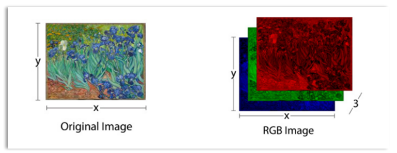
For colored images, each pixel is defined by three color components: red, green, and blue (RGB). Each of these color components is stored as a separate grayscale image, known as a color plane. Together, these three color planes combine to form the full color representation of each pixel in the image.
Pixel values range from 0 to 255, where 0 represents the darkest value (black) and 255 represents the brightest value (white) in the case of grayscale images. To apply algorithms that learn from images, the images must be represented as numerical data, typically in the form of matrices or tensors. These numerical representations allow machine learning models to process and extract patterns from the images.
Matrix and tensor representation of images: Grayscale images
Grayscale images are represented as 3D tensors (equivalent to 3D NumPy arrays). A 3D tensor for a grayscale image has three dimensions:
The first dimension represents the number of samples or images in the dataset.
The second dimension represents the height (number of rows) of the image.
The third dimension represents the width (number of columns) of the image.
Thus, the shape of a grayscale image is represented as (samples, height, width), where samples refers to the number of images, height is the vertical size of the image, and width is the horizontal size of the image.
Let’s randomly generate 2 grayscale images with height=5 and width=5.
Code
1234 )= np.random.randint(low= 0 , high= 255 , size= 50 ).reshape(2 , 5 , 5 )
array([[[ 47, 211,  38,  53, 204],
        [116, 152, 249, 143, 177],
        [ 23, 233, 154,  30, 171],
        [158, 236, 124,  26, 118],
        [186, 120, 112, 220,  69]],

       [[ 80, 201, 127, 246, 254],
        [175,  50, 240, 251,  76],
        [ 37,  34, 166, 250, 195],
        [231, 139, 128, 233,  75],
        [ 80,   3,   2,  19, 140]]])
Code
# shape and dimension of image print ("Image shape: " , images.shape, " \n " ,"Image dimension: " , images.ndim)
Image shape:  (2, 5, 5)
 Image dimension:  3
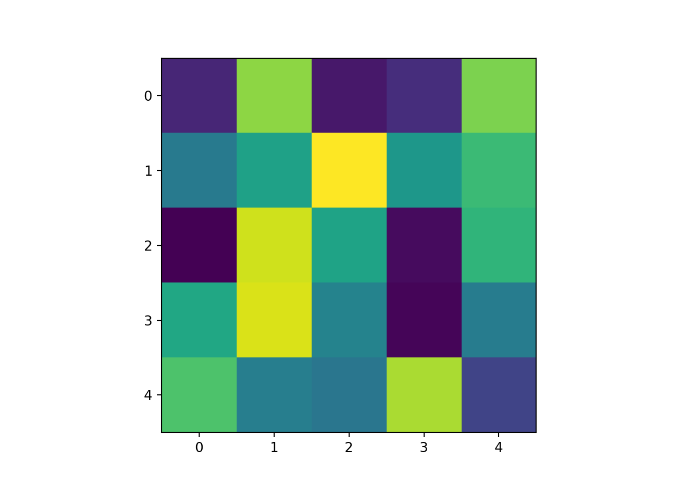
Below is one of the images.
Code
import matplotlib.pyplot as pltprint (images[0 ])
[[ 47 211  38  53 204]
 [116 152 249 143 177]
 [ 23 233 154  30 171]
 [158 236 124  26 118]
 [186 120 112 220  69]]
Code
The 3D image dataset with shape (samples, height, width) can be flattened into a 2D dataset by reshaping each image into a vector. We can reshape the dataset using images.reshape(samples, height * width).
Code
= images.shapeprint ("Samples: " , samples, " \n " ,"Image Height: " , height, " \n " ,"Image Width: " ,width)
Samples:  2
 Image Height:  5
 Image Width:  5
Code
= images.reshape(samples, height* width)
array([[ 47, 211,  38,  53, 204, 116, 152, 249, 143, 177,  23, 233, 154,
         30, 171, 158, 236, 124,  26, 118, 186, 120, 112, 220,  69],
       [ 80, 201, 127, 246, 254, 175,  50, 240, 251,  76,  37,  34, 166,
        250, 195, 231, 139, 128, 233,  75,  80,   3,   2,  19, 140]])
3D Image Datasets (Grayscale Images)
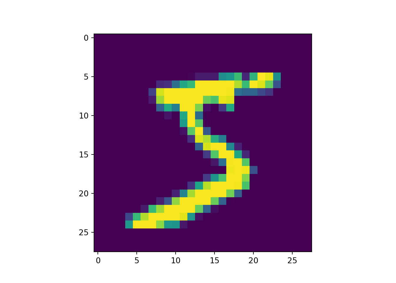
An example of a 3D image dataset is MNIST, which contains 60,000 28x28 grayscale images of the 10 digits, along with a test set of 10,000 images. The MNIST dataset can be loaded using the load_data() function from the keras.datasets module as follows:
Code
from tensorflow.keras.datasets import mnist# Load MNIST dataset = mnist.load_data()# Display shapes of the dataset print (f"Training data shape: { X_train. shape} \n Test data shape: { X_test. shape} " )
Training data shape: (60000, 28, 28)
Test data shape: (10000, 28, 28)
Let’s view the first image in the training set
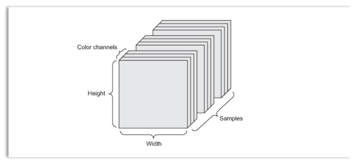
4D Image Datasets (Grayscale Color Images):
Color scale images are represented as 4D tensors with the shape (samples, height, width, color_depth). Each image has a width and height, with three channels representing the red, green, and blue components. In other words, each colored image consists of three grayscale color planes. A 4D color images can be represented as a matrix or tensor.
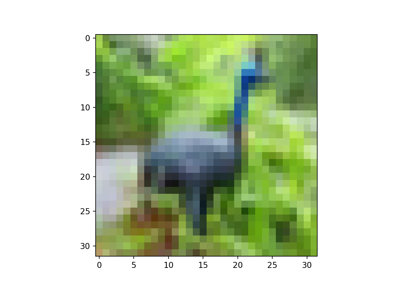
An example of a 4D image dataset is CIFAR-10, which consists of 50,000 32x32 color training images and 10,000 test images, labeled with 10 categories: 0 = airplane; 1 = automobile; 2 = bird; 3 = cat; 4 = deer; 5 = dog; 6 = frog; 7 = horse; 8 = ship; 9 = truck. The CIFAR-10 dataset can be loaded using the .load_data() method from the keras.datasets module..
Code
import ssl# To avoid SSL errors = ssl._create_unverified_context# Load CIFAR-10 dataset from keras.datasets import cifar10= cifar10.load_data()
Downloading data from https://www.cs.toronto.edu/~kriz/cifar-10-python.tar.gz
8192/170498071 [..............................] - ETA: 0s��������������������������������������������������������������
49152/170498071 [..............................] - ETA: 2:54����������������������������������������������������������������
106496/170498071 [..............................] - ETA: 2:50����������������������������������������������������������������
237568/170498071 [..............................] - ETA: 2:22����������������������������������������������������������������
303104/170498071 [..............................] - ETA: 2:19����������������������������������������������������������������
507904/170498071 [..............................] - ETA: 1:48����������������������������������������������������������������
802816/170498071 [..............................] - ETA: 1:25����������������������������������������������������������������
999424/170498071 [..............................] - ETA: 1:17����������������������������������������������������������������
1105920/170498071 [..............................] - ETA: 1:17����������������������������������������������������������������
1269760/170498071 [..............................] - ETA: 1:14����������������������������������������������������������������
1490944/170498071 [..............................] - ETA: 1:12����������������������������������������������������������������
1622016/170498071 [..............................] - ETA: 1:12����������������������������������������������������������������
1818624/170498071 [..............................] - ETA: 1:12����������������������������������������������������������������
1982464/170498071 [..............................] - ETA: 1:10����������������������������������������������������������������
2138112/170498071 [..............................] - ETA: 1:09����������������������������������������������������������������
2154496/170498071 [..............................] - ETA: 1:15����������������������������������������������������������������
2375680/170498071 [..............................] - ETA: 1:13����������������������������������������������������������������
2580480/170498071 [..............................] - ETA: 1:10����������������������������������������������������������������
2809856/170498071 [..............................] - ETA: 1:08����������������������������������������������������������������
3063808/170498071 [..............................] - ETA: 1:05����������������������������������������������������������������
3252224/170498071 [..............................] - ETA: 1:04����������������������������������������������������������������
3547136/170498071 [..............................] - ETA: 1:04����������������������������������������������������������������
3948544/170498071 [..............................] - ETA: 59s ���������������������������������������������������������������
3973120/170498071 [..............................] - ETA: 1:01����������������������������������������������������������������
4341760/170498071 [..............................] - ETA: 58s ���������������������������������������������������������������
4513792/170498071 [..............................] - ETA: 58s���������������������������������������������������������������
4775936/170498071 [..............................] - ETA: 56s���������������������������������������������������������������
4956160/170498071 [..............................] - ETA: 57s���������������������������������������������������������������
5160960/170498071 [..............................] - ETA: 57s���������������������������������������������������������������
5447680/170498071 [..............................] - ETA: 55s���������������������������������������������������������������
5611520/170498071 [..............................] - ETA: 56s���������������������������������������������������������������
5996544/170498071 [>.............................] - ETA: 54s���������������������������������������������������������������
6184960/170498071 [>.............................] - ETA: 53s���������������������������������������������������������������
6438912/170498071 [>.............................] - ETA: 53s���������������������������������������������������������������
6701056/170498071 [>.............................] - ETA: 52s���������������������������������������������������������������
6807552/170498071 [>.............................] - ETA: 53s���������������������������������������������������������������
7028736/170498071 [>.............................] - ETA: 52s���������������������������������������������������������������
7102464/170498071 [>.............................] - ETA: 53s���������������������������������������������������������������
7323648/170498071 [>.............................] - ETA: 52s���������������������������������������������������������������
7593984/170498071 [>.............................] - ETA: 52s���������������������������������������������������������������
7766016/170498071 [>.............................] - ETA: 51s���������������������������������������������������������������
7921664/170498071 [>.............................] - ETA: 51s���������������������������������������������������������������
8175616/170498071 [>.............................] - ETA: 51s���������������������������������������������������������������
8265728/170498071 [>.............................] - ETA: 52s���������������������������������������������������������������
8454144/170498071 [>.............................] - ETA: 51s���������������������������������������������������������������
8683520/170498071 [>.............................] - ETA: 51s���������������������������������������������������������������
8871936/170498071 [>.............................] - ETA: 51s���������������������������������������������������������������
8994816/170498071 [>.............................] - ETA: 51s���������������������������������������������������������������
9117696/170498071 [>.............................] - ETA: 51s���������������������������������������������������������������
9486336/170498071 [>.............................] - ETA: 50s���������������������������������������������������������������
9625600/170498071 [>.............................] - ETA: 50s���������������������������������������������������������������
10010624/170498071 [>.............................] - ETA: 49s���������������������������������������������������������������
10018816/170498071 [>.............................] - ETA: 51s���������������������������������������������������������������
11034624/170498071 [>.............................] - ETA: 48s���������������������������������������������������������������
11198464/170498071 [>.............................] - ETA: 48s���������������������������������������������������������������
11395072/170498071 [=>............................] - ETA: 47s���������������������������������������������������������������
11558912/170498071 [=>............................] - ETA: 47s���������������������������������������������������������������
11747328/170498071 [=>............................] - ETA: 47s���������������������������������������������������������������
12091392/170498071 [=>............................] - ETA: 47s���������������������������������������������������������������
12271616/170498071 [=>............................] - ETA: 47s���������������������������������������������������������������
12509184/170498071 [=>............................] - ETA: 46s���������������������������������������������������������������
12673024/170498071 [=>............................] - ETA: 46s���������������������������������������������������������������
12697600/170498071 [=>............................] - ETA: 47s���������������������������������������������������������������
12959744/170498071 [=>............................] - ETA: 47s���������������������������������������������������������������
13123584/170498071 [=>............................] - ETA: 47s���������������������������������������������������������������
13197312/170498071 [=>............................] - ETA: 47s���������������������������������������������������������������
13271040/170498071 [=>............................] - ETA: 47s���������������������������������������������������������������
13639680/170498071 [=>............................] - ETA: 47s���������������������������������������������������������������
13852672/170498071 [=>............................] - ETA: 46s���������������������������������������������������������������
14172160/170498071 [=>............................] - ETA: 46s���������������������������������������������������������������
14245888/170498071 [=>............................] - ETA: 46s���������������������������������������������������������������
14303232/170498071 [=>............................] - ETA: 47s���������������������������������������������������������������
14508032/170498071 [=>............................] - ETA: 47s���������������������������������������������������������������
14524416/170498071 [=>............................] - ETA: 48s���������������������������������������������������������������
15032320/170498071 [=>............................] - ETA: 47s���������������������������������������������������������������
15106048/170498071 [=>............................] - ETA: 47s���������������������������������������������������������������
15409152/170498071 [=>............................] - ETA: 47s���������������������������������������������������������������
15630336/170498071 [=>............................] - ETA: 47s���������������������������������������������������������������
15958016/170498071 [=>............................] - ETA: 46s���������������������������������������������������������������
16154624/170498071 [=>............................] - ETA: 46s���������������������������������������������������������������
16375808/170498071 [=>............................] - ETA: 46s���������������������������������������������������������������
16654336/170498071 [=>............................] - ETA: 46s���������������������������������������������������������������
17096704/170498071 [==>...........................] - ETA: 46s���������������������������������������������������������������
17170432/170498071 [==>...........................] - ETA: 46s���������������������������������������������������������������
17555456/170498071 [==>...........................] - ETA: 45s���������������������������������������������������������������
17891328/170498071 [==>...........................] - ETA: 45s���������������������������������������������������������������
17997824/170498071 [==>...........................] - ETA: 45s���������������������������������������������������������������
18137088/170498071 [==>...........................] - ETA: 45s���������������������������������������������������������������
18251776/170498071 [==>...........................] - ETA: 45s���������������������������������������������������������������
18366464/170498071 [==>...........................] - ETA: 45s���������������������������������������������������������������
18489344/170498071 [==>...........................] - ETA: 46s���������������������������������������������������������������
18702336/170498071 [==>...........................] - ETA: 46s���������������������������������������������������������������
18890752/170498071 [==>...........................] - ETA: 46s���������������������������������������������������������������
19054592/170498071 [==>...........................] - ETA: 46s���������������������������������������������������������������
19349504/170498071 [==>...........................] - ETA: 45s���������������������������������������������������������������
19439616/170498071 [==>...........................] - ETA: 46s���������������������������������������������������������������
19562496/170498071 [==>...........................] - ETA: 46s���������������������������������������������������������������
19939328/170498071 [==>...........................] - ETA: 45s���������������������������������������������������������������
20013056/170498071 [==>...........................] - ETA: 45s���������������������������������������������������������������
20439040/170498071 [==>...........................] - ETA: 45s���������������������������������������������������������������
20471808/170498071 [==>...........................] - ETA: 46s���������������������������������������������������������������
21086208/170498071 [==>...........................] - ETA: 45s���������������������������������������������������������������
21323776/170498071 [==>...........................] - ETA: 45s���������������������������������������������������������������
21405696/170498071 [==>...........................] - ETA: 45s���������������������������������������������������������������
21512192/170498071 [==>...........................] - ETA: 45s���������������������������������������������������������������
21749760/170498071 [==>...........................] - ETA: 45s���������������������������������������������������������������
21856256/170498071 [==>...........................] - ETA: 45s���������������������������������������������������������������
22110208/170498071 [==>...........................] - ETA: 45s���������������������������������������������������������������
22265856/170498071 [==>...........................] - ETA: 45s���������������������������������������������������������������
22560768/170498071 [==>...........................] - ETA: 44s���������������������������������������������������������������
22626304/170498071 [==>...........................] - ETA: 45s���������������������������������������������������������������
22831104/170498071 [===>..........................] - ETA: 45s���������������������������������������������������������������
22945792/170498071 [===>..........................] - ETA: 45s���������������������������������������������������������������
23207936/170498071 [===>..........................] - ETA: 44s���������������������������������������������������������������
23265280/170498071 [===>..........................] - ETA: 45s���������������������������������������������������������������
23666688/170498071 [===>..........................] - ETA: 45s���������������������������������������������������������������
23846912/170498071 [===>..........................] - ETA: 45s���������������������������������������������������������������
23945216/170498071 [===>..........................] - ETA: 46s���������������������������������������������������������������
24109056/170498071 [===>..........................] - ETA: 46s���������������������������������������������������������������
24305664/170498071 [===>..........................] - ETA: 46s���������������������������������������������������������������
24371200/170498071 [===>..........................] - ETA: 46s���������������������������������������������������������������
24510464/170498071 [===>..........................] - ETA: 46s���������������������������������������������������������������
24600576/170498071 [===>..........................] - ETA: 46s���������������������������������������������������������������
24788992/170498071 [===>..........................] - ETA: 46s���������������������������������������������������������������
24879104/170498071 [===>..........................] - ETA: 46s���������������������������������������������������������������
25051136/170498071 [===>..........................] - ETA: 46s���������������������������������������������������������������
25313280/170498071 [===>..........................] - ETA: 46s���������������������������������������������������������������
25403392/170498071 [===>..........................] - ETA: 46s���������������������������������������������������������������
25608192/170498071 [===>..........................] - ETA: 46s���������������������������������������������������������������
25886720/170498071 [===>..........................] - ETA: 46s���������������������������������������������������������������
26058752/170498071 [===>..........................] - ETA: 46s���������������������������������������������������������������
26238976/170498071 [===>..........................] - ETA: 46s���������������������������������������������������������������
26419200/170498071 [===>..........................] - ETA: 46s���������������������������������������������������������������
26615808/170498071 [===>..........................] - ETA: 46s���������������������������������������������������������������
26746880/170498071 [===>..........................] - ETA: 46s���������������������������������������������������������������
26951680/170498071 [===>..........................] - ETA: 46s���������������������������������������������������������������
27058176/170498071 [===>..........................] - ETA: 46s���������������������������������������������������������������
27230208/170498071 [===>..........................] - ETA: 46s���������������������������������������������������������������
27418624/170498071 [===>..........................] - ETA: 46s���������������������������������������������������������������
27688960/170498071 [===>..........................] - ETA: 45s���������������������������������������������������������������
27795456/170498071 [===>..........................] - ETA: 46s���������������������������������������������������������������
28041216/170498071 [===>..........................] - ETA: 45s���������������������������������������������������������������
28246016/170498071 [===>..........................] - ETA: 45s���������������������������������������������������������������
28409856/170498071 [===>..........................] - ETA: 45s���������������������������������������������������������������
28606464/170498071 [====>.........................] - ETA: 45s���������������������������������������������������������������
28737536/170498071 [====>.........................] - ETA: 45s���������������������������������������������������������������
28958720/170498071 [====>.........................] - ETA: 45s���������������������������������������������������������������
29097984/170498071 [====>.........................] - ETA: 45s���������������������������������������������������������������
29409280/170498071 [====>.........................] - ETA: 45s���������������������������������������������������������������
29605888/170498071 [====>.........................] - ETA: 45s���������������������������������������������������������������
29720576/170498071 [====>.........................] - ETA: 45s���������������������������������������������������������������
29999104/170498071 [====>.........................] - ETA: 44s���������������������������������������������������������������
30031872/170498071 [====>.........................] - ETA: 45s���������������������������������������������������������������
30310400/170498071 [====>.........................] - ETA: 44s���������������������������������������������������������������
30474240/170498071 [====>.........................] - ETA: 44s���������������������������������������������������������������
30703616/170498071 [====>.........................] - ETA: 44s���������������������������������������������������������������
30785536/170498071 [====>.........................] - ETA: 44s���������������������������������������������������������������
31014912/170498071 [====>.........................] - ETA: 44s���������������������������������������������������������������
31096832/170498071 [====>.........................] - ETA: 44s���������������������������������������������������������������
31358976/170498071 [====>.........................] - ETA: 44s���������������������������������������������������������������
31563776/170498071 [====>.........................] - ETA: 44s���������������������������������������������������������������
31612928/170498071 [====>.........................] - ETA: 44s���������������������������������������������������������������
31801344/170498071 [====>.........................] - ETA: 44s���������������������������������������������������������������
31940608/170498071 [====>.........................] - ETA: 44s���������������������������������������������������������������
32202752/170498071 [====>.........................] - ETA: 44s���������������������������������������������������������������
32325632/170498071 [====>.........................] - ETA: 44s���������������������������������������������������������������
32555008/170498071 [====>.........................] - ETA: 44s���������������������������������������������������������������
32833536/170498071 [====>.........................] - ETA: 44s���������������������������������������������������������������
32997376/170498071 [====>.........................] - ETA: 44s���������������������������������������������������������������
33226752/170498071 [====>.........................] - ETA: 44s���������������������������������������������������������������
33406976/170498071 [====>.........................] - ETA: 43s���������������������������������������������������������������
33579008/170498071 [====>.........................] - ETA: 44s���������������������������������������������������������������
33775616/170498071 [====>.........................] - ETA: 44s���������������������������������������������������������������
33890304/170498071 [====>.........................] - ETA: 44s���������������������������������������������������������������
34226176/170498071 [=====>........................] - ETA: 44s���������������������������������������������������������������
34480128/170498071 [=====>........................] - ETA: 43s���������������������������������������������������������������
34529280/170498071 [=====>........................] - ETA: 43s���������������������������������������������������������������
34586624/170498071 [=====>........................] - ETA: 44s���������������������������������������������������������������
34922496/170498071 [=====>........................] - ETA: 44s���������������������������������������������������������������
35127296/170498071 [=====>........................] - ETA: 43s���������������������������������������������������������������
35143680/170498071 [=====>........................] - ETA: 44s���������������������������������������������������������������
35373056/170498071 [=====>........................] - ETA: 44s���������������������������������������������������������������
35520512/170498071 [=====>........................] - ETA: 44s���������������������������������������������������������������
35684352/170498071 [=====>........................] - ETA: 44s���������������������������������������������������������������
35840000/170498071 [=====>........................] - ETA: 44s���������������������������������������������������������������
35979264/170498071 [=====>........................] - ETA: 44s���������������������������������������������������������������
36020224/170498071 [=====>........................] - ETA: 44s���������������������������������������������������������������
36110336/170498071 [=====>........................] - ETA: 44s���������������������������������������������������������������
36274176/170498071 [=====>........................] - ETA: 44s���������������������������������������������������������������
36364288/170498071 [=====>........................] - ETA: 44s���������������������������������������������������������������
36478976/170498071 [=====>........................] - ETA: 44s���������������������������������������������������������������
36626432/170498071 [=====>........................] - ETA: 44s���������������������������������������������������������������
36659200/170498071 [=====>........................] - ETA: 44s���������������������������������������������������������������
36716544/170498071 [=====>........................] - ETA: 44s���������������������������������������������������������������
36864000/170498071 [=====>........................] - ETA: 44s���������������������������������������������������������������
36962304/170498071 [=====>........................] - ETA: 44s���������������������������������������������������������������
37093376/170498071 [=====>........................] - ETA: 45s���������������������������������������������������������������
37208064/170498071 [=====>........................] - ETA: 45s���������������������������������������������������������������
37322752/170498071 [=====>........................] - ETA: 45s���������������������������������������������������������������
37363712/170498071 [=====>........................] - ETA: 45s���������������������������������������������������������������
37494784/170498071 [=====>........................] - ETA: 45s���������������������������������������������������������������
37683200/170498071 [=====>........................] - ETA: 45s���������������������������������������������������������������
37756928/170498071 [=====>........................] - ETA: 45s���������������������������������������������������������������
37855232/170498071 [=====>........................] - ETA: 45s���������������������������������������������������������������
37945344/170498071 [=====>........................] - ETA: 45s���������������������������������������������������������������
38035456/170498071 [=====>........................] - ETA: 46s���������������������������������������������������������������
38133760/170498071 [=====>........................] - ETA: 46s���������������������������������������������������������������
38223872/170498071 [=====>........................] - ETA: 46s���������������������������������������������������������������
38273024/170498071 [=====>........................] - ETA: 46s���������������������������������������������������������������
38371328/170498071 [=====>........................] - ETA: 46s���������������������������������������������������������������
38477824/170498071 [=====>........................] - ETA: 46s���������������������������������������������������������������
38567936/170498071 [=====>........................] - ETA: 46s���������������������������������������������������������������
38674432/170498071 [=====>........................] - ETA: 46s���������������������������������������������������������������
38780928/170498071 [=====>........................] - ETA: 46s���������������������������������������������������������������
38895616/170498071 [=====>........................] - ETA: 46s���������������������������������������������������������������
38993920/170498071 [=====>........................] - ETA: 46s���������������������������������������������������������������
39034880/170498071 [=====>........................] - ETA: 47s���������������������������������������������������������������
39182336/170498071 [=====>........................] - ETA: 46s���������������������������������������������������������������
39256064/170498071 [=====>........................] - ETA: 47s���������������������������������������������������������������
39354368/170498071 [=====>........................] - ETA: 47s���������������������������������������������������������������
39395328/170498071 [=====>........................] - ETA: 47s���������������������������������������������������������������
39469056/170498071 [=====>........................] - ETA: 47s���������������������������������������������������������������
39542784/170498071 [=====>........................] - ETA: 47s���������������������������������������������������������������
39616512/170498071 [=====>........................] - ETA: 47s���������������������������������������������������������������
39706624/170498071 [=====>........................] - ETA: 47s���������������������������������������������������������������
39780352/170498071 [=====>........................] - ETA: 47s���������������������������������������������������������������
39813120/170498071 [======>.......................] - ETA: 47s���������������������������������������������������������������
39903232/170498071 [======>.......................] - ETA: 47s���������������������������������������������������������������
39976960/170498071 [======>.......................] - ETA: 47s���������������������������������������������������������������
40067072/170498071 [======>.......................] - ETA: 48s���������������������������������������������������������������
40148992/170498071 [======>.......................] - ETA: 48s���������������������������������������������������������������
40239104/170498071 [======>.......................] - ETA: 48s���������������������������������������������������������������
40312832/170498071 [======>.......................] - ETA: 48s���������������������������������������������������������������
40386560/170498071 [======>.......................] - ETA: 48s���������������������������������������������������������������
40476672/170498071 [======>.......................] - ETA: 48s���������������������������������������������������������������
40558592/170498071 [======>.......................] - ETA: 48s���������������������������������������������������������������
40640512/170498071 [======>.......................] - ETA: 48s���������������������������������������������������������������
40722432/170498071 [======>.......................] - ETA: 48s���������������������������������������������������������������
40812544/170498071 [======>.......................] - ETA: 48s���������������������������������������������������������������
40902656/170498071 [======>.......................] - ETA: 48s���������������������������������������������������������������
41000960/170498071 [======>.......................] - ETA: 48s���������������������������������������������������������������
41074688/170498071 [======>.......................] - ETA: 48s���������������������������������������������������������������
41164800/170498071 [======>.......................] - ETA: 48s���������������������������������������������������������������
41263104/170498071 [======>.......................] - ETA: 48s���������������������������������������������������������������
41353216/170498071 [======>.......................] - ETA: 48s���������������������������������������������������������������
41451520/170498071 [======>.......................] - ETA: 48s���������������������������������������������������������������
41541632/170498071 [======>.......................] - ETA: 48s���������������������������������������������������������������
41639936/170498071 [======>.......................] - ETA: 48s���������������������������������������������������������������
41730048/170498071 [======>.......................] - ETA: 48s���������������������������������������������������������������
41820160/170498071 [======>.......................] - ETA: 48s���������������������������������������������������������������
41926656/170498071 [======>.......................] - ETA: 48s���������������������������������������������������������������
42008576/170498071 [======>.......................] - ETA: 49s���������������������������������������������������������������
42123264/170498071 [======>.......................] - ETA: 49s���������������������������������������������������������������
42188800/170498071 [======>.......................] - ETA: 49s���������������������������������������������������������������
42254336/170498071 [======>.......................] - ETA: 49s���������������������������������������������������������������
42336256/170498071 [======>.......................] - ETA: 49s���������������������������������������������������������������
42409984/170498071 [======>.......................] - ETA: 49s���������������������������������������������������������������
42483712/170498071 [======>.......................] - ETA: 49s���������������������������������������������������������������
42565632/170498071 [======>.......................] - ETA: 49s���������������������������������������������������������������
42639360/170498071 [======>.......................] - ETA: 49s���������������������������������������������������������������
42713088/170498071 [======>.......................] - ETA: 49s���������������������������������������������������������������
42795008/170498071 [======>.......................] - ETA: 49s���������������������������������������������������������������
42876928/170498071 [======>.......................] - ETA: 49s���������������������������������������������������������������
42942464/170498071 [======>.......................] - ETA: 50s���������������������������������������������������������������
43008000/170498071 [======>.......................] - ETA: 50s���������������������������������������������������������������
43073536/170498071 [======>.......................] - ETA: 50s���������������������������������������������������������������
43171840/170498071 [======>.......................] - ETA: 50s���������������������������������������������������������������
43253760/170498071 [======>.......................] - ETA: 50s���������������������������������������������������������������
43311104/170498071 [======>.......................] - ETA: 50s���������������������������������������������������������������
43376640/170498071 [======>.......................] - ETA: 50s���������������������������������������������������������������
43458560/170498071 [======>.......................] - ETA: 50s���������������������������������������������������������������
43540480/170498071 [======>.......................] - ETA: 50s���������������������������������������������������������������
43548672/170498071 [======>.......................] - ETA: 50s���������������������������������������������������������������
43638784/170498071 [======>.......................] - ETA: 50s���������������������������������������������������������������
43696128/170498071 [======>.......................] - ETA: 51s���������������������������������������������������������������
43753472/170498071 [======>.......................] - ETA: 51s���������������������������������������������������������������
43810816/170498071 [======>.......................] - ETA: 51s���������������������������������������������������������������
43819008/170498071 [======>.......................] - ETA: 51s���������������������������������������������������������������
43884544/170498071 [======>.......................] - ETA: 51s���������������������������������������������������������������
43950080/170498071 [======>.......................] - ETA: 51s���������������������������������������������������������������
43999232/170498071 [======>.......................] - ETA: 51s���������������������������������������������������������������
44007424/170498071 [======>.......................] - ETA: 52s���������������������������������������������������������������
44089344/170498071 [======>.......................] - ETA: 52s���������������������������������������������������������������
44138496/170498071 [======>.......................] - ETA: 52s���������������������������������������������������������������
44187648/170498071 [======>.......................] - ETA: 52s���������������������������������������������������������������
44236800/170498071 [======>.......................] - ETA: 52s���������������������������������������������������������������
44294144/170498071 [======>.......................] - ETA: 52s���������������������������������������������������������������
44351488/170498071 [======>.......................] - ETA: 52s���������������������������������������������������������������
44400640/170498071 [======>.......................] - ETA: 52s���������������������������������������������������������������
44449792/170498071 [======>.......................] - ETA: 52s���������������������������������������������������������������
44507136/170498071 [======>.......................] - ETA: 52s���������������������������������������������������������������
44564480/170498071 [======>.......................] - ETA: 52s���������������������������������������������������������������
44621824/170498071 [======>.......................] - ETA: 53s���������������������������������������������������������������
44687360/170498071 [======>.......................] - ETA: 53s���������������������������������������������������������������
44736512/170498071 [======>.......................] - ETA: 53s���������������������������������������������������������������
44785664/170498071 [======>.......................] - ETA: 53s���������������������������������������������������������������
44843008/170498071 [======>.......................] - ETA: 53s���������������������������������������������������������������
44900352/170498071 [======>.......................] - ETA: 53s���������������������������������������������������������������
44974080/170498071 [======>.......................] - ETA: 53s���������������������������������������������������������������
45039616/170498071 [======>.......................] - ETA: 53s���������������������������������������������������������������
45113344/170498071 [======>.......................] - ETA: 53s���������������������������������������������������������������
45178880/170498071 [======>.......................] - ETA: 53s���������������������������������������������������������������
45244416/170498071 [======>.......................] - ETA: 53s���������������������������������������������������������������
45309952/170498071 [======>.......................] - ETA: 53s���������������������������������������������������������������
45375488/170498071 [======>.......................] - ETA: 53s���������������������������������������������������������������
45424640/170498071 [======>.......................] - ETA: 53s���������������������������������������������������������������
45498368/170498071 [=======>......................] - ETA: 54s���������������������������������������������������������������
45563904/170498071 [=======>......................] - ETA: 54s���������������������������������������������������������������
45637632/170498071 [=======>......................] - ETA: 54s���������������������������������������������������������������
45703168/170498071 [=======>......................] - ETA: 54s���������������������������������������������������������������
45776896/170498071 [=======>......................] - ETA: 54s���������������������������������������������������������������
45858816/170498071 [=======>......................] - ETA: 54s���������������������������������������������������������������
45883392/170498071 [=======>......................] - ETA: 54s���������������������������������������������������������������
45940736/170498071 [=======>......................] - ETA: 54s���������������������������������������������������������������
46014464/170498071 [=======>......................] - ETA: 54s���������������������������������������������������������������
46080000/170498071 [=======>......................] - ETA: 54s���������������������������������������������������������������
46153728/170498071 [=======>......................] - ETA: 54s���������������������������������������������������������������
46227456/170498071 [=======>......................] - ETA: 54s���������������������������������������������������������������
46309376/170498071 [=======>......................] - ETA: 54s���������������������������������������������������������������
46383104/170498071 [=======>......................] - ETA: 54s���������������������������������������������������������������
46456832/170498071 [=======>......................] - ETA: 54s���������������������������������������������������������������
46546944/170498071 [=======>......................] - ETA: 54s���������������������������������������������������������������
46628864/170498071 [=======>......................] - ETA: 54s���������������������������������������������������������������
46694400/170498071 [=======>......................] - ETA: 54s���������������������������������������������������������������
46735360/170498071 [=======>......................] - ETA: 54s���������������������������������������������������������������
46825472/170498071 [=======>......................] - ETA: 54s���������������������������������������������������������������
46891008/170498071 [=======>......................] - ETA: 54s���������������������������������������������������������������
46972928/170498071 [=======>......................] - ETA: 54s���������������������������������������������������������������
47063040/170498071 [=======>......................] - ETA: 54s���������������������������������������������������������������
47136768/170498071 [=======>......................] - ETA: 54s���������������������������������������������������������������
47210496/170498071 [=======>......................] - ETA: 54s���������������������������������������������������������������
47300608/170498071 [=======>......................] - ETA: 54s���������������������������������������������������������������
47382528/170498071 [=======>......................] - ETA: 54s���������������������������������������������������������������
47464448/170498071 [=======>......................] - ETA: 54s���������������������������������������������������������������
47554560/170498071 [=======>......................] - ETA: 54s���������������������������������������������������������������
47652864/170498071 [=======>......................] - ETA: 54s���������������������������������������������������������������
47734784/170498071 [=======>......................] - ETA: 54s���������������������������������������������������������������
47816704/170498071 [=======>......................] - ETA: 54s���������������������������������������������������������������
47906816/170498071 [=======>......................] - ETA: 54s���������������������������������������������������������������
47996928/170498071 [=======>......................] - ETA: 54s���������������������������������������������������������������
48087040/170498071 [=======>......................] - ETA: 54s���������������������������������������������������������������
48177152/170498071 [=======>......................] - ETA: 54s���������������������������������������������������������������
48275456/170498071 [=======>......................] - ETA: 54s���������������������������������������������������������������
48373760/170498071 [=======>......................] - ETA: 54s���������������������������������������������������������������
48398336/170498071 [=======>......................] - ETA: 55s���������������������������������������������������������������
48480256/170498071 [=======>......................] - ETA: 55s���������������������������������������������������������������
48578560/170498071 [=======>......................] - ETA: 55s���������������������������������������������������������������
48644096/170498071 [=======>......................] - ETA: 55s���������������������������������������������������������������
48685056/170498071 [=======>......................] - ETA: 55s���������������������������������������������������������������
48775168/170498071 [=======>......................] - ETA: 55s���������������������������������������������������������������
48865280/170498071 [=======>......................] - ETA: 55s���������������������������������������������������������������
48971776/170498071 [=======>......................] - ETA: 55s���������������������������������������������������������������
49061888/170498071 [=======>......................] - ETA: 55s���������������������������������������������������������������
49127424/170498071 [=======>......................] - ETA: 55s���������������������������������������������������������������
49217536/170498071 [=======>......................] - ETA: 55s���������������������������������������������������������������
49315840/170498071 [=======>......................] - ETA: 55s���������������������������������������������������������������
49397760/170498071 [=======>......................] - ETA: 55s���������������������������������������������������������������
49455104/170498071 [=======>......................] - ETA: 55s���������������������������������������������������������������
49545216/170498071 [=======>......................] - ETA: 55s���������������������������������������������������������������
49610752/170498071 [=======>......................] - ETA: 55s���������������������������������������������������������������
49717248/170498071 [=======>......................] - ETA: 55s���������������������������������������������������������������
49831936/170498071 [=======>......................] - ETA: 55s���������������������������������������������������������������
49938432/170498071 [=======>......................] - ETA: 55s���������������������������������������������������������������
50053120/170498071 [=======>......................] - ETA: 55s���������������������������������������������������������������
50167808/170498071 [=======>......................] - ETA: 55s���������������������������������������������������������������
50274304/170498071 [=======>......................] - ETA: 55s���������������������������������������������������������������
50380800/170498071 [=======>......................] - ETA: 55s���������������������������������������������������������������
50495488/170498071 [=======>......................] - ETA: 55s���������������������������������������������������������������
50601984/170498071 [=======>......................] - ETA: 55s���������������������������������������������������������������
50708480/170498071 [=======>......................] - ETA: 55s���������������������������������������������������������������
50823168/170498071 [=======>......................] - ETA: 55s���������������������������������������������������������������
50929664/170498071 [=======>......................] - ETA: 55s���������������������������������������������������������������
51044352/170498071 [=======>......................] - ETA: 55s���������������������������������������������������������������
51134464/170498071 [=======>......................] - ETA: 54s���������������������������������������������������������������
51224576/170498071 [========>.....................] - ETA: 54s���������������������������������������������������������������
51347456/170498071 [========>.....................] - ETA: 54s���������������������������������������������������������������
51462144/170498071 [========>.....................] - ETA: 54s���������������������������������������������������������������
51576832/170498071 [========>.....................] - ETA: 54s���������������������������������������������������������������
51691520/170498071 [========>.....................] - ETA: 54s���������������������������������������������������������������
51814400/170498071 [========>.....................] - ETA: 54s���������������������������������������������������������������
51929088/170498071 [========>.....................] - ETA: 54s���������������������������������������������������������������
52051968/170498071 [========>.....................] - ETA: 54s���������������������������������������������������������������
52174848/170498071 [========>.....................] - ETA: 54s���������������������������������������������������������������
52289536/170498071 [========>.....................] - ETA: 54s���������������������������������������������������������������
52420608/170498071 [========>.....................] - ETA: 54s���������������������������������������������������������������
52535296/170498071 [========>.....................] - ETA: 54s���������������������������������������������������������������
52658176/170498071 [========>.....................] - ETA: 54s���������������������������������������������������������������
52707328/170498071 [========>.....................] - ETA: 54s���������������������������������������������������������������
52813824/170498071 [========>.....................] - ETA: 54s���������������������������������������������������������������
52928512/170498071 [========>.....................] - ETA: 54s���������������������������������������������������������������
53051392/170498071 [========>.....................] - ETA: 54s���������������������������������������������������������������
53174272/170498071 [========>.....................] - ETA: 54s���������������������������������������������������������������
53231616/170498071 [========>.....................] - ETA: 54s���������������������������������������������������������������
53370880/170498071 [========>.....................] - ETA: 54s���������������������������������������������������������������
53477376/170498071 [========>.....................] - ETA: 54s���������������������������������������������������������������
53600256/170498071 [========>.....................] - ETA: 54s���������������������������������������������������������������
53747712/170498071 [========>.....................] - ETA: 54s���������������������������������������������������������������
53821440/170498071 [========>.....................] - ETA: 54s���������������������������������������������������������������
53903360/170498071 [========>.....................] - ETA: 54s���������������������������������������������������������������
54026240/170498071 [========>.....................] - ETA: 54s���������������������������������������������������������������
54157312/170498071 [========>.....................] - ETA: 54s���������������������������������������������������������������
54288384/170498071 [========>.....................] - ETA: 54s���������������������������������������������������������������
54460416/170498071 [========>.....................] - ETA: 53s���������������������������������������������������������������
54591488/170498071 [========>.....................] - ETA: 53s���������������������������������������������������������������
54697984/170498071 [========>.....................] - ETA: 53s���������������������������������������������������������������
54722560/170498071 [========>.....................] - ETA: 53s���������������������������������������������������������������
54861824/170498071 [========>.....................] - ETA: 53s���������������������������������������������������������������
54992896/170498071 [========>.....................] - ETA: 53s���������������������������������������������������������������
55140352/170498071 [========>.....................] - ETA: 53s���������������������������������������������������������������
55312384/170498071 [========>.....................] - ETA: 53s���������������������������������������������������������������
55410688/170498071 [========>.....................] - ETA: 53s���������������������������������������������������������������
55508992/170498071 [========>.....................] - ETA: 53s���������������������������������������������������������������
55599104/170498071 [========>.....................] - ETA: 53s���������������������������������������������������������������
55697408/170498071 [========>.....................] - ETA: 53s���������������������������������������������������������������
55787520/170498071 [========>.....................] - ETA: 53s���������������������������������������������������������������
55820288/170498071 [========>.....................] - ETA: 53s���������������������������������������������������������������
55902208/170498071 [========>.....................] - ETA: 53s���������������������������������������������������������������
55951360/170498071 [========>.....................] - ETA: 53s���������������������������������������������������������������
56057856/170498071 [========>.....................] - ETA: 53s���������������������������������������������������������������
56172544/170498071 [========>.....................] - ETA: 54s���������������������������������������������������������������
56287232/170498071 [========>.....................] - ETA: 53s���������������������������������������������������������������
56360960/170498071 [========>.....................] - ETA: 54s���������������������������������������������������������������
56426496/170498071 [========>.....................] - ETA: 54s���������������������������������������������������������������
56483840/170498071 [========>.....................] - ETA: 54s���������������������������������������������������������������
56590336/170498071 [========>.....................] - ETA: 54s���������������������������������������������������������������
56655872/170498071 [========>.....................] - ETA: 54s���������������������������������������������������������������
56721408/170498071 [========>.....................] - ETA: 54s���������������������������������������������������������������
56844288/170498071 [=========>....................] - ETA: 54s���������������������������������������������������������������
56868864/170498071 [=========>....................] - ETA: 54s���������������������������������������������������������������
56983552/170498071 [=========>....................] - ETA: 54s���������������������������������������������������������������
57081856/170498071 [=========>....................] - ETA: 54s���������������������������������������������������������������
57106432/170498071 [=========>....................] - ETA: 54s���������������������������������������������������������������
57237504/170498071 [=========>....................] - ETA: 54s���������������������������������������������������������������
57360384/170498071 [=========>....................] - ETA: 54s���������������������������������������������������������������
57491456/170498071 [=========>....................] - ETA: 54s���������������������������������������������������������������
57532416/170498071 [=========>....................] - ETA: 54s���������������������������������������������������������������
57671680/170498071 [=========>....................] - ETA: 54s���������������������������������������������������������������
57794560/170498071 [=========>....................] - ETA: 55s���������������������������������������������������������������
57802752/170498071 [=========>....................] - ETA: 55s���������������������������������������������������������������
57819136/170498071 [=========>....................] - ETA: 55s���������������������������������������������������������������
57851904/170498071 [=========>....................] - ETA: 56s���������������������������������������������������������������
57884672/170498071 [=========>....................] - ETA: 56s���������������������������������������������������������������
57917440/170498071 [=========>....................] - ETA: 56s���������������������������������������������������������������
57966592/170498071 [=========>....................] - ETA: 56s���������������������������������������������������������������
58007552/170498071 [=========>....................] - ETA: 56s���������������������������������������������������������������
58048512/170498071 [=========>....................] - ETA: 56s���������������������������������������������������������������
58089472/170498071 [=========>....................] - ETA: 56s���������������������������������������������������������������
58138624/170498071 [=========>....................] - ETA: 56s���������������������������������������������������������������
58187776/170498071 [=========>....................] - ETA: 56s���������������������������������������������������������������
58245120/170498071 [=========>....................] - ETA: 56s���������������������������������������������������������������
58277888/170498071 [=========>....................] - ETA: 56s���������������������������������������������������������������
58327040/170498071 [=========>....................] - ETA: 56s���������������������������������������������������������������
58384384/170498071 [=========>....................] - ETA: 56s���������������������������������������������������������������
58417152/170498071 [=========>....................] - ETA: 56s���������������������������������������������������������������
58441728/170498071 [=========>....................] - ETA: 56s���������������������������������������������������������������
58474496/170498071 [=========>....................] - ETA: 57s���������������������������������������������������������������
58507264/170498071 [=========>....................] - ETA: 57s���������������������������������������������������������������
58548224/170498071 [=========>....................] - ETA: 57s���������������������������������������������������������������
58572800/170498071 [=========>....................] - ETA: 57s���������������������������������������������������������������
58613760/170498071 [=========>....................] - ETA: 57s���������������������������������������������������������������
58654720/170498071 [=========>....................] - ETA: 57s���������������������������������������������������������������
58679296/170498071 [=========>....................] - ETA: 57s���������������������������������������������������������������
58712064/170498071 [=========>....................] - ETA: 57s���������������������������������������������������������������
58736640/170498071 [=========>....................] - ETA: 57s���������������������������������������������������������������
58761216/170498071 [=========>....................] - ETA: 57s���������������������������������������������������������������
58793984/170498071 [=========>....................] - ETA: 57s���������������������������������������������������������������
58834944/170498071 [=========>....................] - ETA: 57s���������������������������������������������������������������
58875904/170498071 [=========>....................] - ETA: 57s���������������������������������������������������������������
58900480/170498071 [=========>....................] - ETA: 57s���������������������������������������������������������������
58933248/170498071 [=========>....................] - ETA: 57s���������������������������������������������������������������
58974208/170498071 [=========>....................] - ETA: 57s���������������������������������������������������������������
59015168/170498071 [=========>....................] - ETA: 57s���������������������������������������������������������������
59056128/170498071 [=========>....................] - ETA: 57s���������������������������������������������������������������
59088896/170498071 [=========>....................] - ETA: 58s���������������������������������������������������������������
59129856/170498071 [=========>....................] - ETA: 58s���������������������������������������������������������������
59170816/170498071 [=========>....................] - ETA: 58s���������������������������������������������������������������
59219968/170498071 [=========>....................] - ETA: 58s���������������������������������������������������������������
59260928/170498071 [=========>....................] - ETA: 58s���������������������������������������������������������������
59310080/170498071 [=========>....................] - ETA: 58s���������������������������������������������������������������
59359232/170498071 [=========>....................] - ETA: 58s���������������������������������������������������������������
59400192/170498071 [=========>....................] - ETA: 58s���������������������������������������������������������������
59424768/170498071 [=========>....................] - ETA: 58s���������������������������������������������������������������
59490304/170498071 [=========>....................] - ETA: 58s���������������������������������������������������������������
59514880/170498071 [=========>....................] - ETA: 58s���������������������������������������������������������������
59564032/170498071 [=========>....................] - ETA: 58s���������������������������������������������������������������
59621376/170498071 [=========>....................] - ETA: 58s���������������������������������������������������������������
59678720/170498071 [=========>....................] - ETA: 58s���������������������������������������������������������������
59727872/170498071 [=========>....................] - ETA: 58s���������������������������������������������������������������
59777024/170498071 [=========>....................] - ETA: 58s���������������������������������������������������������������
59785216/170498071 [=========>....................] - ETA: 58s���������������������������������������������������������������
59875328/170498071 [=========>....................] - ETA: 58s���������������������������������������������������������������
59916288/170498071 [=========>....................] - ETA: 58s���������������������������������������������������������������
59940864/170498071 [=========>....................] - ETA: 58s���������������������������������������������������������������
59981824/170498071 [=========>....................] - ETA: 58s���������������������������������������������������������������
59998208/170498071 [=========>....................] - ETA: 58s���������������������������������������������������������������
60047360/170498071 [=========>....................] - ETA: 59s���������������������������������������������������������������
60055552/170498071 [=========>....................] - ETA: 59s���������������������������������������������������������������
60063744/170498071 [=========>....................] - ETA: 59s���������������������������������������������������������������
60096512/170498071 [=========>....................] - ETA: 59s���������������������������������������������������������������
60121088/170498071 [=========>....................] - ETA: 59s���������������������������������������������������������������
60153856/170498071 [=========>....................] - ETA: 59s���������������������������������������������������������������
60178432/170498071 [=========>....................] - ETA: 59s���������������������������������������������������������������
60203008/170498071 [=========>....................] - ETA: 59s���������������������������������������������������������������
60235776/170498071 [=========>....................] - ETA: 59s���������������������������������������������������������������
60260352/170498071 [=========>....................] - ETA: 59s���������������������������������������������������������������
60284928/170498071 [=========>....................] - ETA: 59s���������������������������������������������������������������
60309504/170498071 [=========>....................] - ETA: 59s���������������������������������������������������������������
60334080/170498071 [=========>....................] - ETA: 1:00����������������������������������������������������������������
60366848/170498071 [=========>....................] - ETA: 1:00����������������������������������������������������������������
60375040/170498071 [=========>....................] - ETA: 1:00����������������������������������������������������������������
60407808/170498071 [=========>....................] - ETA: 1:00����������������������������������������������������������������
60424192/170498071 [=========>....................] - ETA: 1:00����������������������������������������������������������������
60456960/170498071 [=========>....................] - ETA: 1:00����������������������������������������������������������������
60489728/170498071 [=========>....................] - ETA: 1:00����������������������������������������������������������������
60514304/170498071 [=========>....................] - ETA: 1:00����������������������������������������������������������������
60547072/170498071 [=========>....................] - ETA: 1:00����������������������������������������������������������������
60579840/170498071 [=========>....................] - ETA: 1:00����������������������������������������������������������������
60620800/170498071 [=========>....................] - ETA: 1:00����������������������������������������������������������������
60653568/170498071 [=========>....................] - ETA: 1:00����������������������������������������������������������������
60694528/170498071 [=========>....................] - ETA: 1:00����������������������������������������������������������������
60735488/170498071 [=========>....................] - ETA: 1:00����������������������������������������������������������������
60768256/170498071 [=========>....................] - ETA: 1:00����������������������������������������������������������������
60809216/170498071 [=========>....................] - ETA: 1:00����������������������������������������������������������������
60850176/170498071 [=========>....................] - ETA: 1:00����������������������������������������������������������������
60891136/170498071 [=========>....................] - ETA: 1:00����������������������������������������������������������������
60932096/170498071 [=========>....................] - ETA: 1:00����������������������������������������������������������������
60973056/170498071 [=========>....................] - ETA: 1:01����������������������������������������������������������������
61030400/170498071 [=========>....................] - ETA: 1:01����������������������������������������������������������������
61063168/170498071 [=========>....................] - ETA: 1:01����������������������������������������������������������������
61095936/170498071 [=========>....................] - ETA: 1:01����������������������������������������������������������������
61136896/170498071 [=========>....................] - ETA: 1:01����������������������������������������������������������������
61186048/170498071 [=========>....................] - ETA: 1:01����������������������������������������������������������������
61235200/170498071 [=========>....................] - ETA: 1:01����������������������������������������������������������������
61284352/170498071 [=========>....................] - ETA: 1:01����������������������������������������������������������������
61325312/170498071 [=========>....................] - ETA: 1:01����������������������������������������������������������������
61382656/170498071 [=========>....................] - ETA: 1:01����������������������������������������������������������������
61440000/170498071 [=========>....................] - ETA: 1:01����������������������������������������������������������������
61472768/170498071 [=========>....................] - ETA: 1:01����������������������������������������������������������������
61530112/170498071 [=========>....................] - ETA: 1:01����������������������������������������������������������������
61579264/170498071 [=========>....................] - ETA: 1:01����������������������������������������������������������������
61628416/170498071 [=========>....................] - ETA: 1:01����������������������������������������������������������������
61693952/170498071 [=========>....................] - ETA: 1:01����������������������������������������������������������������
61710336/170498071 [=========>....................] - ETA: 1:01����������������������������������������������������������������
61792256/170498071 [=========>....................] - ETA: 1:01����������������������������������������������������������������
61841408/170498071 [=========>....................] - ETA: 1:01����������������������������������������������������������������
61890560/170498071 [=========>....................] - ETA: 1:01����������������������������������������������������������������
61947904/170498071 [=========>....................] - ETA: 1:01����������������������������������������������������������������
61988864/170498071 [=========>....................] - ETA: 1:01����������������������������������������������������������������
62046208/170498071 [=========>....................] - ETA: 1:01����������������������������������������������������������������
62087168/170498071 [=========>....................] - ETA: 1:01����������������������������������������������������������������
62144512/170498071 [=========>....................] - ETA: 1:01����������������������������������������������������������������
62193664/170498071 [=========>....................] - ETA: 1:01����������������������������������������������������������������
62259200/170498071 [=========>....................] - ETA: 1:01����������������������������������������������������������������
62291968/170498071 [=========>....................] - ETA: 1:02����������������������������������������������������������������
62300160/170498071 [=========>....................] - ETA: 1:02����������������������������������������������������������������
62341120/170498071 [=========>....................] - ETA: 1:02����������������������������������������������������������������
62382080/170498071 [=========>....................] - ETA: 1:02����������������������������������������������������������������
62406656/170498071 [=========>....................] - ETA: 1:02����������������������������������������������������������������
62431232/170498071 [=========>....................] - ETA: 1:02����������������������������������������������������������������
62464000/170498071 [=========>....................] - ETA: 1:02����������������������������������������������������������������
62488576/170498071 [=========>....................] - ETA: 1:02����������������������������������������������������������������
62513152/170498071 [=========>....................] - ETA: 1:02����������������������������������������������������������������
62537728/170498071 [==========>...................] - ETA: 1:02����������������������������������������������������������������
62570496/170498071 [==========>...................] - ETA: 1:02����������������������������������������������������������������
62595072/170498071 [==========>...................] - ETA: 1:02����������������������������������������������������������������
62627840/170498071 [==========>...................] - ETA: 1:02����������������������������������������������������������������
62652416/170498071 [==========>...................] - ETA: 1:03����������������������������������������������������������������
62685184/170498071 [==========>...................] - ETA: 1:03����������������������������������������������������������������
62717952/170498071 [==========>...................] - ETA: 1:03����������������������������������������������������������������
62750720/170498071 [==========>...................] - ETA: 1:03����������������������������������������������������������������
62791680/170498071 [==========>...................] - ETA: 1:03����������������������������������������������������������������
62816256/170498071 [==========>...................] - ETA: 1:03����������������������������������������������������������������
62849024/170498071 [==========>...................] - ETA: 1:03����������������������������������������������������������������
62881792/170498071 [==========>...................] - ETA: 1:03����������������������������������������������������������������
62922752/170498071 [==========>...................] - ETA: 1:03����������������������������������������������������������������
62963712/170498071 [==========>...................] - ETA: 1:03����������������������������������������������������������������
63004672/170498071 [==========>...................] - ETA: 1:03����������������������������������������������������������������
63037440/170498071 [==========>...................] - ETA: 1:03����������������������������������������������������������������
63078400/170498071 [==========>...................] - ETA: 1:03����������������������������������������������������������������
63119360/170498071 [==========>...................] - ETA: 1:03����������������������������������������������������������������
63143936/170498071 [==========>...................] - ETA: 1:03����������������������������������������������������������������
63184896/170498071 [==========>...................] - ETA: 1:03����������������������������������������������������������������
63234048/170498071 [==========>...................] - ETA: 1:03����������������������������������������������������������������
63275008/170498071 [==========>...................] - ETA: 1:03����������������������������������������������������������������
63315968/170498071 [==========>...................] - ETA: 1:03����������������������������������������������������������������
63365120/170498071 [==========>...................] - ETA: 1:04����������������������������������������������������������������
63414272/170498071 [==========>...................] - ETA: 1:04����������������������������������������������������������������
63447040/170498071 [==========>...................] - ETA: 1:04����������������������������������������������������������������
63488000/170498071 [==========>...................] - ETA: 1:04����������������������������������������������������������������
63504384/170498071 [==========>...................] - ETA: 1:04����������������������������������������������������������������
63553536/170498071 [==========>...................] - ETA: 1:04����������������������������������������������������������������
63602688/170498071 [==========>...................] - ETA: 1:04����������������������������������������������������������������
63651840/170498071 [==========>...................] - ETA: 1:04����������������������������������������������������������������
63700992/170498071 [==========>...................] - ETA: 1:04����������������������������������������������������������������
63758336/170498071 [==========>...................] - ETA: 1:04����������������������������������������������������������������
63815680/170498071 [==========>...................] - ETA: 1:04����������������������������������������������������������������
63856640/170498071 [==========>...................] - ETA: 1:04����������������������������������������������������������������
63913984/170498071 [==========>...................] - ETA: 1:04����������������������������������������������������������������
63963136/170498071 [==========>...................] - ETA: 1:04����������������������������������������������������������������
64036864/170498071 [==========>...................] - ETA: 1:04����������������������������������������������������������������
64102400/170498071 [==========>...................] - ETA: 1:04����������������������������������������������������������������
64159744/170498071 [==========>...................] - ETA: 1:04����������������������������������������������������������������
64208896/170498071 [==========>...................] - ETA: 1:04����������������������������������������������������������������
64258048/170498071 [==========>...................] - ETA: 1:04����������������������������������������������������������������
64315392/170498071 [==========>...................] - ETA: 1:04����������������������������������������������������������������
64389120/170498071 [==========>...................] - ETA: 1:04����������������������������������������������������������������
64454656/170498071 [==========>...................] - ETA: 1:04����������������������������������������������������������������
64487424/170498071 [==========>...................] - ETA: 1:04����������������������������������������������������������������
64544768/170498071 [==========>...................] - ETA: 1:04����������������������������������������������������������������
64643072/170498071 [==========>...................] - ETA: 1:04����������������������������������������������������������������
64708608/170498071 [==========>...................] - ETA: 1:04����������������������������������������������������������������
64782336/170498071 [==========>...................] - ETA: 1:04����������������������������������������������������������������
64815104/170498071 [==========>...................] - ETA: 1:04����������������������������������������������������������������
64872448/170498071 [==========>...................] - ETA: 1:04����������������������������������������������������������������
64937984/170498071 [==========>...................] - ETA: 1:04����������������������������������������������������������������
65003520/170498071 [==========>...................] - ETA: 1:04����������������������������������������������������������������
65044480/170498071 [==========>...................] - ETA: 1:04����������������������������������������������������������������
65060864/170498071 [==========>...................] - ETA: 1:04����������������������������������������������������������������
65110016/170498071 [==========>...................] - ETA: 1:04����������������������������������������������������������������
65167360/170498071 [==========>...................] - ETA: 1:04����������������������������������������������������������������
65216512/170498071 [==========>...................] - ETA: 1:04����������������������������������������������������������������
65265664/170498071 [==========>...................] - ETA: 1:04����������������������������������������������������������������
65323008/170498071 [==========>...................] - ETA: 1:04����������������������������������������������������������������
65372160/170498071 [==========>...................] - ETA: 1:04����������������������������������������������������������������
65429504/170498071 [==========>...................] - ETA: 1:04����������������������������������������������������������������
65486848/170498071 [==========>...................] - ETA: 1:04����������������������������������������������������������������
65536000/170498071 [==========>...................] - ETA: 1:04����������������������������������������������������������������
65560576/170498071 [==========>...................] - ETA: 1:04����������������������������������������������������������������
65617920/170498071 [==========>...................] - ETA: 1:05����������������������������������������������������������������
65675264/170498071 [==========>...................] - ETA: 1:05����������������������������������������������������������������
65740800/170498071 [==========>...................] - ETA: 1:05����������������������������������������������������������������
65798144/170498071 [==========>...................] - ETA: 1:05����������������������������������������������������������������
65863680/170498071 [==========>...................] - ETA: 1:05����������������������������������������������������������������
65912832/170498071 [==========>...................] - ETA: 1:05����������������������������������������������������������������
65978368/170498071 [==========>...................] - ETA: 1:05����������������������������������������������������������������
66043904/170498071 [==========>...................] - ETA: 1:05����������������������������������������������������������������
66068480/170498071 [==========>...................] - ETA: 1:05����������������������������������������������������������������
66134016/170498071 [==========>...................] - ETA: 1:05����������������������������������������������������������������
66199552/170498071 [==========>...................] - ETA: 1:05����������������������������������������������������������������
66265088/170498071 [==========>...................] - ETA: 1:05����������������������������������������������������������������
66322432/170498071 [==========>...................] - ETA: 1:05����������������������������������������������������������������
66387968/170498071 [==========>...................] - ETA: 1:05����������������������������������������������������������������
66461696/170498071 [==========>...................] - ETA: 1:05����������������������������������������������������������������
66519040/170498071 [==========>...................] - ETA: 1:05����������������������������������������������������������������
66584576/170498071 [==========>...................] - ETA: 1:05����������������������������������������������������������������
66658304/170498071 [==========>...................] - ETA: 1:05����������������������������������������������������������������
66666496/170498071 [==========>...................] - ETA: 1:05����������������������������������������������������������������
66732032/170498071 [==========>...................] - ETA: 1:05����������������������������������������������������������������
66797568/170498071 [==========>...................] - ETA: 1:05����������������������������������������������������������������
66871296/170498071 [==========>...................] - ETA: 1:05����������������������������������������������������������������
66928640/170498071 [==========>...................] - ETA: 1:05����������������������������������������������������������������
66994176/170498071 [==========>...................] - ETA: 1:05����������������������������������������������������������������
67067904/170498071 [==========>...................] - ETA: 1:05����������������������������������������������������������������
67141632/170498071 [==========>...................] - ETA: 1:05����������������������������������������������������������������
67215360/170498071 [==========>...................] - ETA: 1:05����������������������������������������������������������������
67280896/170498071 [==========>...................] - ETA: 1:05����������������������������������������������������������������
67354624/170498071 [==========>...................] - ETA: 1:05����������������������������������������������������������������
67428352/170498071 [==========>...................] - ETA: 1:05����������������������������������������������������������������
67502080/170498071 [==========>...................] - ETA: 1:05����������������������������������������������������������������
67575808/170498071 [==========>...................] - ETA: 1:05����������������������������������������������������������������
67649536/170498071 [==========>...................] - ETA: 1:04����������������������������������������������������������������
67723264/170498071 [==========>...................] - ETA: 1:05����������������������������������������������������������������
67805184/170498071 [==========>...................] - ETA: 1:05����������������������������������������������������������������
67887104/170498071 [==========>...................] - ETA: 1:04����������������������������������������������������������������
67960832/170498071 [==========>...................] - ETA: 1:04����������������������������������������������������������������
68050944/170498071 [==========>...................] - ETA: 1:04����������������������������������������������������������������
68132864/170498071 [==========>...................] - ETA: 1:04����������������������������������������������������������������
68198400/170498071 [==========>...................] - ETA: 1:04����������������������������������������������������������������
68280320/170498071 [===========>..................] - ETA: 1:04����������������������������������������������������������������
68362240/170498071 [===========>..................] - ETA: 1:04����������������������������������������������������������������
68444160/170498071 [===========>..................] - ETA: 1:04����������������������������������������������������������������
68542464/170498071 [===========>..................] - ETA: 1:04����������������������������������������������������������������
68608000/170498071 [===========>..................] - ETA: 1:04����������������������������������������������������������������
68632576/170498071 [===========>..................] - ETA: 1:04����������������������������������������������������������������
68722688/170498071 [===========>..................] - ETA: 1:04����������������������������������������������������������������
68812800/170498071 [===========>..................] - ETA: 1:04����������������������������������������������������������������
68902912/170498071 [===========>..................] - ETA: 1:04����������������������������������������������������������������
68952064/170498071 [===========>..................] - ETA: 1:04����������������������������������������������������������������
69042176/170498071 [===========>..................] - ETA: 1:04����������������������������������������������������������������
69115904/170498071 [===========>..................] - ETA: 1:04����������������������������������������������������������������
69148672/170498071 [===========>..................] - ETA: 1:04����������������������������������������������������������������
69238784/170498071 [===========>..................] - ETA: 1:04����������������������������������������������������������������
69328896/170498071 [===========>..................] - ETA: 1:04����������������������������������������������������������������
69419008/170498071 [===========>..................] - ETA: 1:04����������������������������������������������������������������
69509120/170498071 [===========>..................] - ETA: 1:04����������������������������������������������������������������
69566464/170498071 [===========>..................] - ETA: 1:04����������������������������������������������������������������
69648384/170498071 [===========>..................] - ETA: 1:04����������������������������������������������������������������
69746688/170498071 [===========>..................] - ETA: 1:04����������������������������������������������������������������
69836800/170498071 [===========>..................] - ETA: 1:04����������������������������������������������������������������
69935104/170498071 [===========>..................] - ETA: 1:04����������������������������������������������������������������
70017024/170498071 [===========>..................] - ETA: 1:04����������������������������������������������������������������
70123520/170498071 [===========>..................] - ETA: 1:03����������������������������������������������������������������
70221824/170498071 [===========>..................] - ETA: 1:03����������������������������������������������������������������
70320128/170498071 [===========>..................] - ETA: 1:03����������������������������������������������������������������
70418432/170498071 [===========>..................] - ETA: 1:03����������������������������������������������������������������
70557696/170498071 [===========>..................] - ETA: 1:03����������������������������������������������������������������
70631424/170498071 [===========>..................] - ETA: 1:03����������������������������������������������������������������
70696960/170498071 [===========>..................] - ETA: 1:03����������������������������������������������������������������
70770688/170498071 [===========>..................] - ETA: 1:03����������������������������������������������������������������
70852608/170498071 [===========>..................] - ETA: 1:03����������������������������������������������������������������
70926336/170498071 [===========>..................] - ETA: 1:03����������������������������������������������������������������
70975488/170498071 [===========>..................] - ETA: 1:03����������������������������������������������������������������
71024640/170498071 [===========>..................] - ETA: 1:03����������������������������������������������������������������
71081984/170498071 [===========>..................] - ETA: 1:03����������������������������������������������������������������
71131136/170498071 [===========>..................] - ETA: 1:03����������������������������������������������������������������
71188480/170498071 [===========>..................] - ETA: 1:03����������������������������������������������������������������
71254016/170498071 [===========>..................] - ETA: 1:03����������������������������������������������������������������
71303168/170498071 [===========>..................] - ETA: 1:03����������������������������������������������������������������
71327744/170498071 [===========>..................] - ETA: 1:03����������������������������������������������������������������
71376896/170498071 [===========>..................] - ETA: 1:03����������������������������������������������������������������
71417856/170498071 [===========>..................] - ETA: 1:03����������������������������������������������������������������
71467008/170498071 [===========>..................] - ETA: 1:03����������������������������������������������������������������
71507968/170498071 [===========>..................] - ETA: 1:03����������������������������������������������������������������
71557120/170498071 [===========>..................] - ETA: 1:03����������������������������������������������������������������
71598080/170498071 [===========>..................] - ETA: 1:03����������������������������������������������������������������
71655424/170498071 [===========>..................] - ETA: 1:03����������������������������������������������������������������
71680000/170498071 [===========>..................] - ETA: 1:03����������������������������������������������������������������
71729152/170498071 [===========>..................] - ETA: 1:04����������������������������������������������������������������
71778304/170498071 [===========>..................] - ETA: 1:04����������������������������������������������������������������
71827456/170498071 [===========>..................] - ETA: 1:04����������������������������������������������������������������
71884800/170498071 [===========>..................] - ETA: 1:04����������������������������������������������������������������
71925760/170498071 [===========>..................] - ETA: 1:04����������������������������������������������������������������
71974912/170498071 [===========>..................] - ETA: 1:04����������������������������������������������������������������
72024064/170498071 [===========>..................] - ETA: 1:04����������������������������������������������������������������
72081408/170498071 [===========>..................] - ETA: 1:04����������������������������������������������������������������
72138752/170498071 [===========>..................] - ETA: 1:04����������������������������������������������������������������
72196096/170498071 [===========>..................] - ETA: 1:04����������������������������������������������������������������
72237056/170498071 [===========>..................] - ETA: 1:04����������������������������������������������������������������
72294400/170498071 [===========>..................] - ETA: 1:04����������������������������������������������������������������
72335360/170498071 [===========>..................] - ETA: 1:04����������������������������������������������������������������
72368128/170498071 [===========>..................] - ETA: 1:04����������������������������������������������������������������
72409088/170498071 [===========>..................] - ETA: 1:04����������������������������������������������������������������
72441856/170498071 [===========>..................] - ETA: 1:04����������������������������������������������������������������
72507392/170498071 [===========>..................] - ETA: 1:04����������������������������������������������������������������
72540160/170498071 [===========>..................] - ETA: 1:04����������������������������������������������������������������
72572928/170498071 [===========>..................] - ETA: 1:04����������������������������������������������������������������
72613888/170498071 [===========>..................] - ETA: 1:04����������������������������������������������������������������
72646656/170498071 [===========>..................] - ETA: 1:04����������������������������������������������������������������
72679424/170498071 [===========>..................] - ETA: 1:04����������������������������������������������������������������
72704000/170498071 [===========>..................] - ETA: 1:04����������������������������������������������������������������
72744960/170498071 [===========>..................] - ETA: 1:04����������������������������������������������������������������
72753152/170498071 [===========>..................] - ETA: 1:04����������������������������������������������������������������
72785920/170498071 [===========>..................] - ETA: 1:04����������������������������������������������������������������
72826880/170498071 [===========>..................] - ETA: 1:05����������������������������������������������������������������
72859648/170498071 [===========>..................] - ETA: 1:05����������������������������������������������������������������
72900608/170498071 [===========>..................] - ETA: 1:05����������������������������������������������������������������
72933376/170498071 [===========>..................] - ETA: 1:05����������������������������������������������������������������
72949760/170498071 [===========>..................] - ETA: 1:05����������������������������������������������������������������
72982528/170498071 [===========>..................] - ETA: 1:05����������������������������������������������������������������
73023488/170498071 [===========>..................] - ETA: 1:05����������������������������������������������������������������
73056256/170498071 [===========>..................] - ETA: 1:05����������������������������������������������������������������
73064448/170498071 [===========>..................] - ETA: 1:05����������������������������������������������������������������
73121792/170498071 [===========>..................] - ETA: 1:05����������������������������������������������������������������
73154560/170498071 [===========>..................] - ETA: 1:05����������������������������������������������������������������
73179136/170498071 [===========>..................] - ETA: 1:05����������������������������������������������������������������
73203712/170498071 [===========>..................] - ETA: 1:05����������������������������������������������������������������
73228288/170498071 [===========>..................] - ETA: 1:05����������������������������������������������������������������
73252864/170498071 [===========>..................] - ETA: 1:05����������������������������������������������������������������
73277440/170498071 [===========>..................] - ETA: 1:05����������������������������������������������������������������
73310208/170498071 [===========>..................] - ETA: 1:05����������������������������������������������������������������
73334784/170498071 [===========>..................] - ETA: 1:05����������������������������������������������������������������
73342976/170498071 [===========>..................] - ETA: 1:05����������������������������������������������������������������
73375744/170498071 [===========>..................] - ETA: 1:05����������������������������������������������������������������
73392128/170498071 [===========>..................] - ETA: 1:06����������������������������������������������������������������
73416704/170498071 [===========>..................] - ETA: 1:06����������������������������������������������������������������
73449472/170498071 [===========>..................] - ETA: 1:06����������������������������������������������������������������
73474048/170498071 [===========>..................] - ETA: 1:06����������������������������������������������������������������
73506816/170498071 [===========>..................] - ETA: 1:06����������������������������������������������������������������
73531392/170498071 [===========>..................] - ETA: 1:06����������������������������������������������������������������
73564160/170498071 [===========>..................] - ETA: 1:06����������������������������������������������������������������
73605120/170498071 [===========>..................] - ETA: 1:06����������������������������������������������������������������
73621504/170498071 [===========>..................] - ETA: 1:06����������������������������������������������������������������
73654272/170498071 [===========>..................] - ETA: 1:06����������������������������������������������������������������
73678848/170498071 [===========>..................] - ETA: 1:06����������������������������������������������������������������
73711616/170498071 [===========>..................] - ETA: 1:06����������������������������������������������������������������
73736192/170498071 [===========>..................] - ETA: 1:06����������������������������������������������������������������
73777152/170498071 [===========>..................] - ETA: 1:06����������������������������������������������������������������
73826304/170498071 [===========>..................] - ETA: 1:06����������������������������������������������������������������
73859072/170498071 [===========>..................] - ETA: 1:06����������������������������������������������������������������
73891840/170498071 [============>.................] - ETA: 1:06����������������������������������������������������������������
73932800/170498071 [============>.................] - ETA: 1:06����������������������������������������������������������������
73973760/170498071 [============>.................] - ETA: 1:06����������������������������������������������������������������
74014720/170498071 [============>.................] - ETA: 1:06����������������������������������������������������������������
74055680/170498071 [============>.................] - ETA: 1:06����������������������������������������������������������������
74096640/170498071 [============>.................] - ETA: 1:06����������������������������������������������������������������
74121216/170498071 [============>.................] - ETA: 1:06����������������������������������������������������������������
74129408/170498071 [============>.................] - ETA: 1:06����������������������������������������������������������������
74178560/170498071 [============>.................] - ETA: 1:06����������������������������������������������������������������
74219520/170498071 [============>.................] - ETA: 1:06����������������������������������������������������������������
74260480/170498071 [============>.................] - ETA: 1:06����������������������������������������������������������������
74309632/170498071 [============>.................] - ETA: 1:06����������������������������������������������������������������
74326016/170498071 [============>.................] - ETA: 1:06����������������������������������������������������������������
74383360/170498071 [============>.................] - ETA: 1:06����������������������������������������������������������������
74407936/170498071 [============>.................] - ETA: 1:06����������������������������������������������������������������
74448896/170498071 [============>.................] - ETA: 1:07����������������������������������������������������������������
74481664/170498071 [============>.................] - ETA: 1:07����������������������������������������������������������������
74522624/170498071 [============>.................] - ETA: 1:07����������������������������������������������������������������
74563584/170498071 [============>.................] - ETA: 1:07����������������������������������������������������������������
74596352/170498071 [============>.................] - ETA: 1:07����������������������������������������������������������������
74637312/170498071 [============>.................] - ETA: 1:07����������������������������������������������������������������
74678272/170498071 [============>.................] - ETA: 1:07����������������������������������������������������������������
74702848/170498071 [============>.................] - ETA: 1:07����������������������������������������������������������������
74743808/170498071 [============>.................] - ETA: 1:07����������������������������������������������������������������
74760192/170498071 [============>.................] - ETA: 1:07����������������������������������������������������������������
74801152/170498071 [============>.................] - ETA: 1:07����������������������������������������������������������������
74850304/170498071 [============>.................] - ETA: 1:07����������������������������������������������������������������
74891264/170498071 [============>.................] - ETA: 1:07����������������������������������������������������������������
74932224/170498071 [============>.................] - ETA: 1:07����������������������������������������������������������������
74973184/170498071 [============>.................] - ETA: 1:07����������������������������������������������������������������
74997760/170498071 [============>.................] - ETA: 1:07����������������������������������������������������������������
75030528/170498071 [============>.................] - ETA: 1:07����������������������������������������������������������������
75071488/170498071 [============>.................] - ETA: 1:07����������������������������������������������������������������
75112448/170498071 [============>.................] - ETA: 1:07����������������������������������������������������������������
75161600/170498071 [============>.................] - ETA: 1:07����������������������������������������������������������������
75202560/170498071 [============>.................] - ETA: 1:07����������������������������������������������������������������
75276288/170498071 [============>.................] - ETA: 1:07����������������������������������������������������������������
75309056/170498071 [============>.................] - ETA: 1:07����������������������������������������������������������������
75333632/170498071 [============>.................] - ETA: 1:07����������������������������������������������������������������
75366400/170498071 [============>.................] - ETA: 1:07����������������������������������������������������������������
75399168/170498071 [============>.................] - ETA: 1:07����������������������������������������������������������������
75431936/170498071 [============>.................] - ETA: 1:07����������������������������������������������������������������
75464704/170498071 [============>.................] - ETA: 1:07����������������������������������������������������������������
75505664/170498071 [============>.................] - ETA: 1:07����������������������������������������������������������������
75546624/170498071 [============>.................] - ETA: 1:07����������������������������������������������������������������
75571200/170498071 [============>.................] - ETA: 1:07����������������������������������������������������������������
75603968/170498071 [============>.................] - ETA: 1:07����������������������������������������������������������������
75644928/170498071 [============>.................] - ETA: 1:07����������������������������������������������������������������
75669504/170498071 [============>.................] - ETA: 1:07����������������������������������������������������������������
75710464/170498071 [============>.................] - ETA: 1:07����������������������������������������������������������������
75743232/170498071 [============>.................] - ETA: 1:07����������������������������������������������������������������
75767808/170498071 [============>.................] - ETA: 1:07����������������������������������������������������������������
75792384/170498071 [============>.................] - ETA: 1:07����������������������������������������������������������������
75825152/170498071 [============>.................] - ETA: 1:07����������������������������������������������������������������
75857920/170498071 [============>.................] - ETA: 1:07����������������������������������������������������������������
75882496/170498071 [============>.................] - ETA: 1:07����������������������������������������������������������������
75915264/170498071 [============>.................] - ETA: 1:07����������������������������������������������������������������
75948032/170498071 [============>.................] - ETA: 1:08����������������������������������������������������������������
75980800/170498071 [============>.................] - ETA: 1:08����������������������������������������������������������������
76021760/170498071 [============>.................] - ETA: 1:08����������������������������������������������������������������
76062720/170498071 [============>.................] - ETA: 1:08����������������������������������������������������������������
76095488/170498071 [============>.................] - ETA: 1:08����������������������������������������������������������������
76120064/170498071 [============>.................] - ETA: 1:08����������������������������������������������������������������
76161024/170498071 [============>.................] - ETA: 1:08����������������������������������������������������������������
76201984/170498071 [============>.................] - ETA: 1:08����������������������������������������������������������������
76242944/170498071 [============>.................] - ETA: 1:08����������������������������������������������������������������
76292096/170498071 [============>.................] - ETA: 1:08����������������������������������������������������������������
76349440/170498071 [============>.................] - ETA: 1:08����������������������������������������������������������������
76390400/170498071 [============>.................] - ETA: 1:08����������������������������������������������������������������
76439552/170498071 [============>.................] - ETA: 1:08����������������������������������������������������������������
76472320/170498071 [============>.................] - ETA: 1:08����������������������������������������������������������������
76513280/170498071 [============>.................] - ETA: 1:08����������������������������������������������������������������
76554240/170498071 [============>.................] - ETA: 1:08����������������������������������������������������������������
76611584/170498071 [============>.................] - ETA: 1:08����������������������������������������������������������������
76660736/170498071 [============>.................] - ETA: 1:08����������������������������������������������������������������
76709888/170498071 [============>.................] - ETA: 1:08����������������������������������������������������������������
76759040/170498071 [============>.................] - ETA: 1:08����������������������������������������������������������������
76800000/170498071 [============>.................] - ETA: 1:08����������������������������������������������������������������
76849152/170498071 [============>.................] - ETA: 1:08����������������������������������������������������������������
76906496/170498071 [============>.................] - ETA: 1:08����������������������������������������������������������������
76955648/170498071 [============>.................] - ETA: 1:08����������������������������������������������������������������
76972032/170498071 [============>.................] - ETA: 1:08����������������������������������������������������������������
77029376/170498071 [============>.................] - ETA: 1:08����������������������������������������������������������������
77053952/170498071 [============>.................] - ETA: 1:08����������������������������������������������������������������
77094912/170498071 [============>.................] - ETA: 1:08����������������������������������������������������������������
77144064/170498071 [============>.................] - ETA: 1:08����������������������������������������������������������������
77185024/170498071 [============>.................] - ETA: 1:08����������������������������������������������������������������
77225984/170498071 [============>.................] - ETA: 1:08����������������������������������������������������������������
77275136/170498071 [============>.................] - ETA: 1:08����������������������������������������������������������������
77316096/170498071 [============>.................] - ETA: 1:08����������������������������������������������������������������
77365248/170498071 [============>.................] - ETA: 1:08����������������������������������������������������������������
77414400/170498071 [============>.................] - ETA: 1:08����������������������������������������������������������������
77455360/170498071 [============>.................] - ETA: 1:08����������������������������������������������������������������
77496320/170498071 [============>.................] - ETA: 1:08����������������������������������������������������������������
77545472/170498071 [============>.................] - ETA: 1:08����������������������������������������������������������������
77594624/170498071 [============>.................] - ETA: 1:08����������������������������������������������������������������
77635584/170498071 [============>.................] - ETA: 1:08����������������������������������������������������������������
77684736/170498071 [============>.................] - ETA: 1:08����������������������������������������������������������������
77709312/170498071 [============>.................] - ETA: 1:08����������������������������������������������������������������
77758464/170498071 [============>.................] - ETA: 1:08����������������������������������������������������������������
77807616/170498071 [============>.................] - ETA: 1:08����������������������������������������������������������������
77848576/170498071 [============>.................] - ETA: 1:08����������������������������������������������������������������
77897728/170498071 [============>.................] - ETA: 1:08����������������������������������������������������������������
77946880/170498071 [============>.................] - ETA: 1:08����������������������������������������������������������������
78004224/170498071 [============>.................] - ETA: 1:08����������������������������������������������������������������
78036992/170498071 [============>.................] - ETA: 1:08����������������������������������������������������������������
78069760/170498071 [============>.................] - ETA: 1:08����������������������������������������������������������������
78127104/170498071 [============>.................] - ETA: 1:08����������������������������������������������������������������
78176256/170498071 [============>.................] - ETA: 1:08����������������������������������������������������������������
78233600/170498071 [============>.................] - ETA: 1:08����������������������������������������������������������������
78290944/170498071 [============>.................] - ETA: 1:08����������������������������������������������������������������
78299136/170498071 [============>.................] - ETA: 1:08����������������������������������������������������������������
78381056/170498071 [============>.................] - ETA: 1:08����������������������������������������������������������������
78397440/170498071 [============>.................] - ETA: 1:08����������������������������������������������������������������
78446592/170498071 [============>.................] - ETA: 1:08����������������������������������������������������������������
78487552/170498071 [============>.................] - ETA: 1:08����������������������������������������������������������������
78528512/170498071 [============>.................] - ETA: 1:08����������������������������������������������������������������
78577664/170498071 [============>.................] - ETA: 1:08����������������������������������������������������������������
78585856/170498071 [============>.................] - ETA: 1:08����������������������������������������������������������������
78643200/170498071 [============>.................] - ETA: 1:08����������������������������������������������������������������
78675968/170498071 [============>.................] - ETA: 1:08����������������������������������������������������������������
78716928/170498071 [============>.................] - ETA: 1:08����������������������������������������������������������������
78749696/170498071 [============>.................] - ETA: 1:09����������������������������������������������������������������
78782464/170498071 [============>.................] - ETA: 1:09����������������������������������������������������������������
78831616/170498071 [============>.................] - ETA: 1:09����������������������������������������������������������������
78856192/170498071 [============>.................] - ETA: 1:09����������������������������������������������������������������
78897152/170498071 [============>.................] - ETA: 1:09����������������������������������������������������������������
78929920/170498071 [============>.................] - ETA: 1:09����������������������������������������������������������������
78970880/170498071 [============>.................] - ETA: 1:09����������������������������������������������������������������
79011840/170498071 [============>.................] - ETA: 1:09����������������������������������������������������������������
79044608/170498071 [============>.................] - ETA: 1:09����������������������������������������������������������������
79085568/170498071 [============>.................] - ETA: 1:09����������������������������������������������������������������
79101952/170498071 [============>.................] - ETA: 1:09����������������������������������������������������������������
79142912/170498071 [============>.................] - ETA: 1:09����������������������������������������������������������������
79183872/170498071 [============>.................] - ETA: 1:09����������������������������������������������������������������
79216640/170498071 [============>.................] - ETA: 1:09����������������������������������������������������������������
79265792/170498071 [============>.................] - ETA: 1:09����������������������������������������������������������������
79323136/170498071 [============>.................] - ETA: 1:09����������������������������������������������������������������
79364096/170498071 [============>.................] - ETA: 1:09����������������������������������������������������������������
79413248/170498071 [============>.................] - ETA: 1:09����������������������������������������������������������������
79462400/170498071 [============>.................] - ETA: 1:09����������������������������������������������������������������
79519744/170498071 [============>.................] - ETA: 1:09����������������������������������������������������������������
79560704/170498071 [============>.................] - ETA: 1:09����������������������������������������������������������������
79609856/170498071 [=============>................] - ETA: 1:09����������������������������������������������������������������
79675392/170498071 [=============>................] - ETA: 1:09����������������������������������������������������������������
79732736/170498071 [=============>................] - ETA: 1:09����������������������������������������������������������������
79773696/170498071 [=============>................] - ETA: 1:09����������������������������������������������������������������
79814656/170498071 [=============>................] - ETA: 1:09����������������������������������������������������������������
79863808/170498071 [=============>................] - ETA: 1:09����������������������������������������������������������������
79880192/170498071 [=============>................] - ETA: 1:09����������������������������������������������������������������
79904768/170498071 [=============>................] - ETA: 1:09����������������������������������������������������������������
79937536/170498071 [=============>................] - ETA: 1:09����������������������������������������������������������������
79986688/170498071 [=============>................] - ETA: 1:09����������������������������������������������������������������
80044032/170498071 [=============>................] - ETA: 1:09����������������������������������������������������������������
80068608/170498071 [=============>................] - ETA: 1:09����������������������������������������������������������������
80134144/170498071 [=============>................] - ETA: 1:09����������������������������������������������������������������
80175104/170498071 [=============>................] - ETA: 1:09����������������������������������������������������������������
80199680/170498071 [=============>................] - ETA: 1:09����������������������������������������������������������������
80216064/170498071 [=============>................] - ETA: 1:09����������������������������������������������������������������
80240640/170498071 [=============>................] - ETA: 1:09����������������������������������������������������������������
80289792/170498071 [=============>................] - ETA: 1:09����������������������������������������������������������������
80314368/170498071 [=============>................] - ETA: 1:09����������������������������������������������������������������
80338944/170498071 [=============>................] - ETA: 1:09����������������������������������������������������������������
80371712/170498071 [=============>................] - ETA: 1:09����������������������������������������������������������������
80396288/170498071 [=============>................] - ETA: 1:09����������������������������������������������������������������
80420864/170498071 [=============>................] - ETA: 1:09����������������������������������������������������������������
80453632/170498071 [=============>................] - ETA: 1:09����������������������������������������������������������������
80486400/170498071 [=============>................] - ETA: 1:09����������������������������������������������������������������
80510976/170498071 [=============>................] - ETA: 1:09����������������������������������������������������������������
80543744/170498071 [=============>................] - ETA: 1:09����������������������������������������������������������������
80576512/170498071 [=============>................] - ETA: 1:09����������������������������������������������������������������
80609280/170498071 [=============>................] - ETA: 1:09����������������������������������������������������������������
80633856/170498071 [=============>................] - ETA: 1:09����������������������������������������������������������������
80674816/170498071 [=============>................] - ETA: 1:09����������������������������������������������������������������
80699392/170498071 [=============>................] - ETA: 1:09����������������������������������������������������������������
80748544/170498071 [=============>................] - ETA: 1:09����������������������������������������������������������������
80773120/170498071 [=============>................] - ETA: 1:09����������������������������������������������������������������
80805888/170498071 [=============>................] - ETA: 1:09����������������������������������������������������������������
80838656/170498071 [=============>................] - ETA: 1:09����������������������������������������������������������������
80863232/170498071 [=============>................] - ETA: 1:09����������������������������������������������������������������
80896000/170498071 [=============>................] - ETA: 1:09����������������������������������������������������������������
80928768/170498071 [=============>................] - ETA: 1:09����������������������������������������������������������������
80961536/170498071 [=============>................] - ETA: 1:09����������������������������������������������������������������
80994304/170498071 [=============>................] - ETA: 1:09����������������������������������������������������������������
81035264/170498071 [=============>................] - ETA: 1:09����������������������������������������������������������������
81059840/170498071 [=============>................] - ETA: 1:09����������������������������������������������������������������
81100800/170498071 [=============>................] - ETA: 1:09����������������������������������������������������������������
81133568/170498071 [=============>................] - ETA: 1:09����������������������������������������������������������������
81174528/170498071 [=============>................] - ETA: 1:09����������������������������������������������������������������
81207296/170498071 [=============>................] - ETA: 1:09����������������������������������������������������������������
81240064/170498071 [=============>................] - ETA: 1:09����������������������������������������������������������������
81272832/170498071 [=============>................] - ETA: 1:09����������������������������������������������������������������
81289216/170498071 [=============>................] - ETA: 1:09����������������������������������������������������������������
81330176/170498071 [=============>................] - ETA: 1:09����������������������������������������������������������������
81362944/170498071 [=============>................] - ETA: 1:09����������������������������������������������������������������
81403904/170498071 [=============>................] - ETA: 1:09����������������������������������������������������������������
81444864/170498071 [=============>................] - ETA: 1:09����������������������������������������������������������������
81485824/170498071 [=============>................] - ETA: 1:09����������������������������������������������������������������
81534976/170498071 [=============>................] - ETA: 1:09����������������������������������������������������������������
81575936/170498071 [=============>................] - ETA: 1:09����������������������������������������������������������������
81616896/170498071 [=============>................] - ETA: 1:09����������������������������������������������������������������
81666048/170498071 [=============>................] - ETA: 1:09����������������������������������������������������������������
81715200/170498071 [=============>................] - ETA: 1:09����������������������������������������������������������������
81764352/170498071 [=============>................] - ETA: 1:09����������������������������������������������������������������
81813504/170498071 [=============>................] - ETA: 1:09����������������������������������������������������������������
81862656/170498071 [=============>................] - ETA: 1:09����������������������������������������������������������������
81911808/170498071 [=============>................] - ETA: 1:09����������������������������������������������������������������
81960960/170498071 [=============>................] - ETA: 1:09����������������������������������������������������������������
82026496/170498071 [=============>................] - ETA: 1:09����������������������������������������������������������������
82083840/170498071 [=============>................] - ETA: 1:09����������������������������������������������������������������
82124800/170498071 [=============>................] - ETA: 1:09����������������������������������������������������������������
82173952/170498071 [=============>................] - ETA: 1:09����������������������������������������������������������������
82231296/170498071 [=============>................] - ETA: 1:09����������������������������������������������������������������
82280448/170498071 [=============>................] - ETA: 1:09����������������������������������������������������������������
82329600/170498071 [=============>................] - ETA: 1:09����������������������������������������������������������������
82378752/170498071 [=============>................] - ETA: 1:09����������������������������������������������������������������
82427904/170498071 [=============>................] - ETA: 1:09����������������������������������������������������������������
82485248/170498071 [=============>................] - ETA: 1:09����������������������������������������������������������������
82550784/170498071 [=============>................] - ETA: 1:09����������������������������������������������������������������
82608128/170498071 [=============>................] - ETA: 1:09����������������������������������������������������������������
82665472/170498071 [=============>................] - ETA: 1:09����������������������������������������������������������������
82739200/170498071 [=============>................] - ETA: 1:09����������������������������������������������������������������
82788352/170498071 [=============>................] - ETA: 1:09����������������������������������������������������������������
82862080/170498071 [=============>................] - ETA: 1:09����������������������������������������������������������������
82919424/170498071 [=============>................] - ETA: 1:09����������������������������������������������������������������
82960384/170498071 [=============>................] - ETA: 1:09����������������������������������������������������������������
83042304/170498071 [=============>................] - ETA: 1:09����������������������������������������������������������������
83116032/170498071 [=============>................] - ETA: 1:09����������������������������������������������������������������
83189760/170498071 [=============>................] - ETA: 1:09����������������������������������������������������������������
83247104/170498071 [=============>................] - ETA: 1:08����������������������������������������������������������������
83304448/170498071 [=============>................] - ETA: 1:08����������������������������������������������������������������
83369984/170498071 [=============>................] - ETA: 1:08����������������������������������������������������������������
83435520/170498071 [=============>................] - ETA: 1:08����������������������������������������������������������������
83509248/170498071 [=============>................] - ETA: 1:08����������������������������������������������������������������
83550208/170498071 [=============>................] - ETA: 1:08����������������������������������������������������������������
83591168/170498071 [=============>................] - ETA: 1:08����������������������������������������������������������������
83632128/170498071 [=============>................] - ETA: 1:08����������������������������������������������������������������
83681280/170498071 [=============>................] - ETA: 1:08����������������������������������������������������������������
83738624/170498071 [=============>................] - ETA: 1:08����������������������������������������������������������������
83804160/170498071 [=============>................] - ETA: 1:08����������������������������������������������������������������
83836928/170498071 [=============>................] - ETA: 1:08����������������������������������������������������������������
83886080/170498071 [=============>................] - ETA: 1:08����������������������������������������������������������������
83935232/170498071 [=============>................] - ETA: 1:08����������������������������������������������������������������
83984384/170498071 [=============>................] - ETA: 1:08����������������������������������������������������������������
84041728/170498071 [=============>................] - ETA: 1:08����������������������������������������������������������������
84099072/170498071 [=============>................] - ETA: 1:08����������������������������������������������������������������
84164608/170498071 [=============>................] - ETA: 1:08����������������������������������������������������������������
84205568/170498071 [=============>................] - ETA: 1:08����������������������������������������������������������������
84271104/170498071 [=============>................] - ETA: 1:08����������������������������������������������������������������
84328448/170498071 [=============>................] - ETA: 1:08����������������������������������������������������������������
84385792/170498071 [=============>................] - ETA: 1:08����������������������������������������������������������������
84418560/170498071 [=============>................] - ETA: 1:08����������������������������������������������������������������
84467712/170498071 [=============>................] - ETA: 1:08����������������������������������������������������������������
84533248/170498071 [=============>................] - ETA: 1:08����������������������������������������������������������������
84598784/170498071 [=============>................] - ETA: 1:08����������������������������������������������������������������
84647936/170498071 [=============>................] - ETA: 1:08����������������������������������������������������������������
84713472/170498071 [=============>................] - ETA: 1:08����������������������������������������������������������������
84770816/170498071 [=============>................] - ETA: 1:08����������������������������������������������������������������
84836352/170498071 [=============>................] - ETA: 1:08����������������������������������������������������������������
84852736/170498071 [=============>................] - ETA: 1:08����������������������������������������������������������������
84918272/170498071 [=============>................] - ETA: 1:08����������������������������������������������������������������
84959232/170498071 [=============>................] - ETA: 1:08����������������������������������������������������������������
85008384/170498071 [=============>................] - ETA: 1:08����������������������������������������������������������������
85082112/170498071 [=============>................] - ETA: 1:08����������������������������������������������������������������
85106688/170498071 [=============>................] - ETA: 1:08����������������������������������������������������������������
85155840/170498071 [=============>................] - ETA: 1:08����������������������������������������������������������������
85221376/170498071 [=============>................] - ETA: 1:08����������������������������������������������������������������
85303296/170498071 [==============>...............] - ETA: 1:08����������������������������������������������������������������
85344256/170498071 [==============>...............] - ETA: 1:08����������������������������������������������������������������
85393408/170498071 [==============>...............] - ETA: 1:08����������������������������������������������������������������
85442560/170498071 [==============>...............] - ETA: 1:08����������������������������������������������������������������
85499904/170498071 [==============>...............] - ETA: 1:08����������������������������������������������������������������
85549056/170498071 [==============>...............] - ETA: 1:08����������������������������������������������������������������
85557248/170498071 [==============>...............] - ETA: 1:08����������������������������������������������������������������
85606400/170498071 [==============>...............] - ETA: 1:08����������������������������������������������������������������
85663744/170498071 [==============>...............] - ETA: 1:08����������������������������������������������������������������
85712896/170498071 [==============>...............] - ETA: 1:08����������������������������������������������������������������
85745664/170498071 [==============>...............] - ETA: 1:08����������������������������������������������������������������
85794816/170498071 [==============>...............] - ETA: 1:08����������������������������������������������������������������
85852160/170498071 [==============>...............] - ETA: 1:08����������������������������������������������������������������
85917696/170498071 [==============>...............] - ETA: 1:08����������������������������������������������������������������
85975040/170498071 [==============>...............] - ETA: 1:08����������������������������������������������������������������
86024192/170498071 [==============>...............] - ETA: 1:08����������������������������������������������������������������
86130688/170498071 [==============>...............] - ETA: 1:08����������������������������������������������������������������
86171648/170498071 [==============>...............] - ETA: 1:08����������������������������������������������������������������
86212608/170498071 [==============>...............] - ETA: 1:07����������������������������������������������������������������
86253568/170498071 [==============>...............] - ETA: 1:08����������������������������������������������������������������
86310912/170498071 [==============>...............] - ETA: 1:07����������������������������������������������������������������
86351872/170498071 [==============>...............] - ETA: 1:07����������������������������������������������������������������
86401024/170498071 [==============>...............] - ETA: 1:07����������������������������������������������������������������
86450176/170498071 [==============>...............] - ETA: 1:07����������������������������������������������������������������
86491136/170498071 [==============>...............] - ETA: 1:07����������������������������������������������������������������
86540288/170498071 [==============>...............] - ETA: 1:07����������������������������������������������������������������
86597632/170498071 [==============>...............] - ETA: 1:07����������������������������������������������������������������
86654976/170498071 [==============>...............] - ETA: 1:07����������������������������������������������������������������
86695936/170498071 [==============>...............] - ETA: 1:07����������������������������������������������������������������
86720512/170498071 [==============>...............] - ETA: 1:07����������������������������������������������������������������
86769664/170498071 [==============>...............] - ETA: 1:07����������������������������������������������������������������
86827008/170498071 [==============>...............] - ETA: 1:07����������������������������������������������������������������
86876160/170498071 [==============>...............] - ETA: 1:07����������������������������������������������������������������
86933504/170498071 [==============>...............] - ETA: 1:07����������������������������������������������������������������
86982656/170498071 [==============>...............] - ETA: 1:07����������������������������������������������������������������
87040000/170498071 [==============>...............] - ETA: 1:07����������������������������������������������������������������
87097344/170498071 [==============>...............] - ETA: 1:07����������������������������������������������������������������
87154688/170498071 [==============>...............] - ETA: 1:07����������������������������������������������������������������
87212032/170498071 [==============>...............] - ETA: 1:07����������������������������������������������������������������
87261184/170498071 [==============>...............] - ETA: 1:07����������������������������������������������������������������
87302144/170498071 [==============>...............] - ETA: 1:07����������������������������������������������������������������
87334912/170498071 [==============>...............] - ETA: 1:07����������������������������������������������������������������
87375872/170498071 [==============>...............] - ETA: 1:07����������������������������������������������������������������
87408640/170498071 [==============>...............] - ETA: 1:07����������������������������������������������������������������
87457792/170498071 [==============>...............] - ETA: 1:07����������������������������������������������������������������
87506944/170498071 [==============>...............] - ETA: 1:07����������������������������������������������������������������
87556096/170498071 [==============>...............] - ETA: 1:07����������������������������������������������������������������
87613440/170498071 [==============>...............] - ETA: 1:07����������������������������������������������������������������
87654400/170498071 [==============>...............] - ETA: 1:07����������������������������������������������������������������
87703552/170498071 [==============>...............] - ETA: 1:07����������������������������������������������������������������
87744512/170498071 [==============>...............] - ETA: 1:07����������������������������������������������������������������
87793664/170498071 [==============>...............] - ETA: 1:07����������������������������������������������������������������
87842816/170498071 [==============>...............] - ETA: 1:07����������������������������������������������������������������
87900160/170498071 [==============>...............] - ETA: 1:07����������������������������������������������������������������
87949312/170498071 [==============>...............] - ETA: 1:07����������������������������������������������������������������
88006656/170498071 [==============>...............] - ETA: 1:07����������������������������������������������������������������
88055808/170498071 [==============>...............] - ETA: 1:07����������������������������������������������������������������
88104960/170498071 [==============>...............] - ETA: 1:07����������������������������������������������������������������
88154112/170498071 [==============>...............] - ETA: 1:07����������������������������������������������������������������
88211456/170498071 [==============>...............] - ETA: 1:07����������������������������������������������������������������
88268800/170498071 [==============>...............] - ETA: 1:07����������������������������������������������������������������
88326144/170498071 [==============>...............] - ETA: 1:07����������������������������������������������������������������
88391680/170498071 [==============>...............] - ETA: 1:07����������������������������������������������������������������
88449024/170498071 [==============>...............] - ETA: 1:07����������������������������������������������������������������
88498176/170498071 [==============>...............] - ETA: 1:07����������������������������������������������������������������
88555520/170498071 [==============>...............] - ETA: 1:07����������������������������������������������������������������
88612864/170498071 [==============>...............] - ETA: 1:07����������������������������������������������������������������
88678400/170498071 [==============>...............] - ETA: 1:07����������������������������������������������������������������
88735744/170498071 [==============>...............] - ETA: 1:07����������������������������������������������������������������
88793088/170498071 [==============>...............] - ETA: 1:07����������������������������������������������������������������
88858624/170498071 [==============>...............] - ETA: 1:07����������������������������������������������������������������
88924160/170498071 [==============>...............] - ETA: 1:07����������������������������������������������������������������
88981504/170498071 [==============>...............] - ETA: 1:07����������������������������������������������������������������
89047040/170498071 [==============>...............] - ETA: 1:06����������������������������������������������������������������
89120768/170498071 [==============>...............] - ETA: 1:06����������������������������������������������������������������
89186304/170498071 [==============>...............] - ETA: 1:06����������������������������������������������������������������
89260032/170498071 [==============>...............] - ETA: 1:06����������������������������������������������������������������
89325568/170498071 [==============>...............] - ETA: 1:06����������������������������������������������������������������
89391104/170498071 [==============>...............] - ETA: 1:06����������������������������������������������������������������
89448448/170498071 [==============>...............] - ETA: 1:06����������������������������������������������������������������
89522176/170498071 [==============>...............] - ETA: 1:06����������������������������������������������������������������
89595904/170498071 [==============>...............] - ETA: 1:06����������������������������������������������������������������
89661440/170498071 [==============>...............] - ETA: 1:06����������������������������������������������������������������
89735168/170498071 [==============>...............] - ETA: 1:06����������������������������������������������������������������
89808896/170498071 [==============>...............] - ETA: 1:06����������������������������������������������������������������
89849856/170498071 [==============>...............] - ETA: 1:06����������������������������������������������������������������
89890816/170498071 [==============>...............] - ETA: 1:06����������������������������������������������������������������
89964544/170498071 [==============>...............] - ETA: 1:06����������������������������������������������������������������
90038272/170498071 [==============>...............] - ETA: 1:06����������������������������������������������������������������
90112000/170498071 [==============>...............] - ETA: 1:06����������������������������������������������������������������
90193920/170498071 [==============>...............] - ETA: 1:06����������������������������������������������������������������
90259456/170498071 [==============>...............] - ETA: 1:06����������������������������������������������������������������
90324992/170498071 [==============>...............] - ETA: 1:05����������������������������������������������������������������
90382336/170498071 [==============>...............] - ETA: 1:05����������������������������������������������������������������
90456064/170498071 [==============>...............] - ETA: 1:05����������������������������������������������������������������
90546176/170498071 [==============>...............] - ETA: 1:05����������������������������������������������������������������
90628096/170498071 [==============>...............] - ETA: 1:05����������������������������������������������������������������
90685440/170498071 [==============>...............] - ETA: 1:05����������������������������������������������������������������
90718208/170498071 [==============>...............] - ETA: 1:05����������������������������������������������������������������
90791936/170498071 [==============>...............] - ETA: 1:05����������������������������������������������������������������
90882048/170498071 [==============>...............] - ETA: 1:05����������������������������������������������������������������
90980352/170498071 [===============>..............] - ETA: 1:05����������������������������������������������������������������
91070464/170498071 [===============>..............] - ETA: 1:05����������������������������������������������������������������
91144192/170498071 [===============>..............] - ETA: 1:05����������������������������������������������������������������
91168768/170498071 [===============>..............] - ETA: 1:05����������������������������������������������������������������
91267072/170498071 [===============>..............] - ETA: 1:05����������������������������������������������������������������
91357184/170498071 [===============>..............] - ETA: 1:05����������������������������������������������������������������
91422720/170498071 [===============>..............] - ETA: 1:04����������������������������������������������������������������
91504640/170498071 [===============>..............] - ETA: 1:04����������������������������������������������������������������
91586560/170498071 [===============>..............] - ETA: 1:04����������������������������������������������������������������
91660288/170498071 [===============>..............] - ETA: 1:04����������������������������������������������������������������
91742208/170498071 [===============>..............] - ETA: 1:04����������������������������������������������������������������
91824128/170498071 [===============>..............] - ETA: 1:04����������������������������������������������������������������
91897856/170498071 [===============>..............] - ETA: 1:04����������������������������������������������������������������
91987968/170498071 [===============>..............] - ETA: 1:04����������������������������������������������������������������
92061696/170498071 [===============>..............] - ETA: 1:04����������������������������������������������������������������
92102656/170498071 [===============>..............] - ETA: 1:04����������������������������������������������������������������
92192768/170498071 [===============>..............] - ETA: 1:04����������������������������������������������������������������
92291072/170498071 [===============>..............] - ETA: 1:04����������������������������������������������������������������
92381184/170498071 [===============>..............] - ETA: 1:04����������������������������������������������������������������
92405760/170498071 [===============>..............] - ETA: 1:04����������������������������������������������������������������
92504064/170498071 [===============>..............] - ETA: 1:04����������������������������������������������������������������
92528640/170498071 [===============>..............] - ETA: 1:04����������������������������������������������������������������
92594176/170498071 [===============>..............] - ETA: 1:03����������������������������������������������������������������
92651520/170498071 [===============>..............] - ETA: 1:03����������������������������������������������������������������
92749824/170498071 [===============>..............] - ETA: 1:03����������������������������������������������������������������
92839936/170498071 [===============>..............] - ETA: 1:03����������������������������������������������������������������
92954624/170498071 [===============>..............] - ETA: 1:03����������������������������������������������������������������
93044736/170498071 [===============>..............] - ETA: 1:03����������������������������������������������������������������
93151232/170498071 [===============>..............] - ETA: 1:03����������������������������������������������������������������
93241344/170498071 [===============>..............] - ETA: 1:03����������������������������������������������������������������
93347840/170498071 [===============>..............] - ETA: 1:03����������������������������������������������������������������
93454336/170498071 [===============>..............] - ETA: 1:03����������������������������������������������������������������
93552640/170498071 [===============>..............] - ETA: 1:03����������������������������������������������������������������
93659136/170498071 [===============>..............] - ETA: 1:03����������������������������������������������������������������
93765632/170498071 [===============>..............] - ETA: 1:03����������������������������������������������������������������
93888512/170498071 [===============>..............] - ETA: 1:02����������������������������������������������������������������
93970432/170498071 [===============>..............] - ETA: 1:02����������������������������������������������������������������
94052352/170498071 [===============>..............] - ETA: 1:02����������������������������������������������������������������
94109696/170498071 [===============>..............] - ETA: 1:02����������������������������������������������������������������
94134272/170498071 [===============>..............] - ETA: 1:02����������������������������������������������������������������
94208000/170498071 [===============>..............] - ETA: 1:02����������������������������������������������������������������
94257152/170498071 [===============>..............] - ETA: 1:02����������������������������������������������������������������
94330880/170498071 [===============>..............] - ETA: 1:02����������������������������������������������������������������
94388224/170498071 [===============>..............] - ETA: 1:02����������������������������������������������������������������
94470144/170498071 [===============>..............] - ETA: 1:02����������������������������������������������������������������
94552064/170498071 [===============>..............] - ETA: 1:02����������������������������������������������������������������
94617600/170498071 [===============>..............] - ETA: 1:02����������������������������������������������������������������
94691328/170498071 [===============>..............] - ETA: 1:02����������������������������������������������������������������
94707712/170498071 [===============>..............] - ETA: 1:02����������������������������������������������������������������
94797824/170498071 [===============>..............] - ETA: 1:02����������������������������������������������������������������
94863360/170498071 [===============>..............] - ETA: 1:02����������������������������������������������������������������
94945280/170498071 [===============>..............] - ETA: 1:02����������������������������������������������������������������
95035392/170498071 [===============>..............] - ETA: 1:02����������������������������������������������������������������
95076352/170498071 [===============>..............] - ETA: 1:02����������������������������������������������������������������
95133696/170498071 [===============>..............] - ETA: 1:02����������������������������������������������������������������
95232000/170498071 [===============>..............] - ETA: 1:01����������������������������������������������������������������
95330304/170498071 [===============>..............] - ETA: 1:01����������������������������������������������������������������
95412224/170498071 [===============>..............] - ETA: 1:01����������������������������������������������������������������
95477760/170498071 [===============>..............] - ETA: 1:01����������������������������������������������������������������
95559680/170498071 [===============>..............] - ETA: 1:01����������������������������������������������������������������
95657984/170498071 [===============>..............] - ETA: 1:01����������������������������������������������������������������
95748096/170498071 [===============>..............] - ETA: 1:01����������������������������������������������������������������
95764480/170498071 [===============>..............] - ETA: 1:01����������������������������������������������������������������
95862784/170498071 [===============>..............] - ETA: 1:01����������������������������������������������������������������
95870976/170498071 [===============>..............] - ETA: 1:01����������������������������������������������������������������
95977472/170498071 [===============>..............] - ETA: 1:01����������������������������������������������������������������
96051200/170498071 [===============>..............] - ETA: 1:01����������������������������������������������������������������
96075776/170498071 [===============>..............] - ETA: 1:01����������������������������������������������������������������
96223232/170498071 [===============>..............] - ETA: 1:01����������������������������������������������������������������
96288768/170498071 [===============>..............] - ETA: 1:01����������������������������������������������������������������
96321536/170498071 [===============>..............] - ETA: 1:01����������������������������������������������������������������
96395264/170498071 [===============>..............] - ETA: 1:01����������������������������������������������������������������
96468992/170498071 [===============>..............] - ETA: 1:01����������������������������������������������������������������
96493568/170498071 [===============>..............] - ETA: 1:01����������������������������������������������������������������
96567296/170498071 [===============>..............] - ETA: 1:01����������������������������������������������������������������
96591872/170498071 [===============>..............] - ETA: 1:01����������������������������������������������������������������
96665600/170498071 [================>.............] - ETA: 1:01����������������������������������������������������������������
96722944/170498071 [================>.............] - ETA: 1:01����������������������������������������������������������������
96837632/170498071 [================>.............] - ETA: 1:00����������������������������������������������������������������
96911360/170498071 [================>.............] - ETA: 1:00����������������������������������������������������������������
96960512/170498071 [================>.............] - ETA: 1:00����������������������������������������������������������������
97017856/170498071 [================>.............] - ETA: 1:00����������������������������������������������������������������
97042432/170498071 [================>.............] - ETA: 1:00����������������������������������������������������������������
97050624/170498071 [================>.............] - ETA: 1:00����������������������������������������������������������������
97140736/170498071 [================>.............] - ETA: 1:00����������������������������������������������������������������
97181696/170498071 [================>.............] - ETA: 1:00����������������������������������������������������������������
97206272/170498071 [================>.............] - ETA: 1:00����������������������������������������������������������������
97222656/170498071 [================>.............] - ETA: 1:00����������������������������������������������������������������
97271808/170498071 [================>.............] - ETA: 1:00����������������������������������������������������������������
97312768/170498071 [================>.............] - ETA: 1:00����������������������������������������������������������������
97361920/170498071 [================>.............] - ETA: 1:00����������������������������������������������������������������
97386496/170498071 [================>.............] - ETA: 1:00����������������������������������������������������������������
97435648/170498071 [================>.............] - ETA: 1:00����������������������������������������������������������������
97452032/170498071 [================>.............] - ETA: 1:00����������������������������������������������������������������
97533952/170498071 [================>.............] - ETA: 1:00����������������������������������������������������������������
97566720/170498071 [================>.............] - ETA: 1:00����������������������������������������������������������������
97607680/170498071 [================>.............] - ETA: 1:00����������������������������������������������������������������
97640448/170498071 [================>.............] - ETA: 1:00����������������������������������������������������������������
97681408/170498071 [================>.............] - ETA: 1:00����������������������������������������������������������������
97722368/170498071 [================>.............] - ETA: 1:00����������������������������������������������������������������
97763328/170498071 [================>.............] - ETA: 1:00����������������������������������������������������������������
97796096/170498071 [================>.............] - ETA: 1:00����������������������������������������������������������������
97837056/170498071 [================>.............] - ETA: 1:00����������������������������������������������������������������
97878016/170498071 [================>.............] - ETA: 1:00����������������������������������������������������������������
97918976/170498071 [================>.............] - ETA: 1:00����������������������������������������������������������������
97959936/170498071 [================>.............] - ETA: 1:00����������������������������������������������������������������
97984512/170498071 [================>.............] - ETA: 1:00����������������������������������������������������������������
98025472/170498071 [================>.............] - ETA: 1:00����������������������������������������������������������������
98074624/170498071 [================>.............] - ETA: 1:00����������������������������������������������������������������
98115584/170498071 [================>.............] - ETA: 1:00����������������������������������������������������������������
98156544/170498071 [================>.............] - ETA: 1:00����������������������������������������������������������������
98205696/170498071 [================>.............] - ETA: 1:00����������������������������������������������������������������
98246656/170498071 [================>.............] - ETA: 1:00����������������������������������������������������������������
98295808/170498071 [================>.............] - ETA: 1:00����������������������������������������������������������������
98328576/170498071 [================>.............] - ETA: 1:00����������������������������������������������������������������
98385920/170498071 [================>.............] - ETA: 1:00����������������������������������������������������������������
98435072/170498071 [================>.............] - ETA: 1:00����������������������������������������������������������������
98476032/170498071 [================>.............] - ETA: 1:00����������������������������������������������������������������
98557952/170498071 [================>.............] - ETA: 1:00����������������������������������������������������������������
98590720/170498071 [================>.............] - ETA: 1:00����������������������������������������������������������������
98623488/170498071 [================>.............] - ETA: 1:00����������������������������������������������������������������
98656256/170498071 [================>.............] - ETA: 1:00����������������������������������������������������������������
98705408/170498071 [================>.............] - ETA: 1:00����������������������������������������������������������������
98729984/170498071 [================>.............] - ETA: 1:00����������������������������������������������������������������
98770944/170498071 [================>.............] - ETA: 1:00����������������������������������������������������������������
98820096/170498071 [================>.............] - ETA: 1:00����������������������������������������������������������������
98861056/170498071 [================>.............] - ETA: 1:00����������������������������������������������������������������
98902016/170498071 [================>.............] - ETA: 1:00����������������������������������������������������������������
98942976/170498071 [================>.............] - ETA: 1:00����������������������������������������������������������������
98983936/170498071 [================>.............] - ETA: 1:00����������������������������������������������������������������
99024896/170498071 [================>.............] - ETA: 1:00����������������������������������������������������������������
99074048/170498071 [================>.............] - ETA: 1:00����������������������������������������������������������������
99131392/170498071 [================>.............] - ETA: 1:00����������������������������������������������������������������
99172352/170498071 [================>.............] - ETA: 1:00����������������������������������������������������������������
99221504/170498071 [================>.............] - ETA: 1:00����������������������������������������������������������������
99262464/170498071 [================>.............] - ETA: 1:00����������������������������������������������������������������
99311616/170498071 [================>.............] - ETA: 1:00����������������������������������������������������������������
99360768/170498071 [================>.............] - ETA: 1:00����������������������������������������������������������������
99409920/170498071 [================>.............] - ETA: 59s ���������������������������������������������������������������
99467264/170498071 [================>.............] - ETA: 59s���������������������������������������������������������������
99524608/170498071 [================>.............] - ETA: 59s���������������������������������������������������������������
99573760/170498071 [================>.............] - ETA: 59s���������������������������������������������������������������
99614720/170498071 [================>.............] - ETA: 59s���������������������������������������������������������������
99672064/170498071 [================>.............] - ETA: 59s���������������������������������������������������������������
99721216/170498071 [================>.............] - ETA: 59s���������������������������������������������������������������
99778560/170498071 [================>.............] - ETA: 59s���������������������������������������������������������������
99827712/170498071 [================>.............] - ETA: 59s���������������������������������������������������������������
99876864/170498071 [================>.............] - ETA: 59s���������������������������������������������������������������
99926016/170498071 [================>.............] - ETA: 59s���������������������������������������������������������������
99983360/170498071 [================>.............] - ETA: 59s���������������������������������������������������������������
100032512/170498071 [================>.............] - ETA: 59s���������������������������������������������������������������
100098048/170498071 [================>.............] - ETA: 59s���������������������������������������������������������������
100155392/170498071 [================>.............] - ETA: 59s���������������������������������������������������������������
100212736/170498071 [================>.............] - ETA: 59s���������������������������������������������������������������
100294656/170498071 [================>.............] - ETA: 59s���������������������������������������������������������������
100352000/170498071 [================>.............] - ETA: 59s���������������������������������������������������������������
100417536/170498071 [================>.............] - ETA: 59s���������������������������������������������������������������
100474880/170498071 [================>.............] - ETA: 59s���������������������������������������������������������������
100532224/170498071 [================>.............] - ETA: 59s���������������������������������������������������������������
100597760/170498071 [================>.............] - ETA: 59s���������������������������������������������������������������
100663296/170498071 [================>.............] - ETA: 59s���������������������������������������������������������������
100728832/170498071 [================>.............] - ETA: 59s���������������������������������������������������������������
100786176/170498071 [================>.............] - ETA: 59s���������������������������������������������������������������
100827136/170498071 [================>.............] - ETA: 58s���������������������������������������������������������������
100892672/170498071 [================>.............] - ETA: 58s���������������������������������������������������������������
100966400/170498071 [================>.............] - ETA: 58s���������������������������������������������������������������
101031936/170498071 [================>.............] - ETA: 58s���������������������������������������������������������������
101097472/170498071 [================>.............] - ETA: 58s���������������������������������������������������������������
101171200/170498071 [================>.............] - ETA: 58s���������������������������������������������������������������
101244928/170498071 [================>.............] - ETA: 58s���������������������������������������������������������������
101318656/170498071 [================>.............] - ETA: 58s���������������������������������������������������������������
101359616/170498071 [================>.............] - ETA: 58s���������������������������������������������������������������
101408768/170498071 [================>.............] - ETA: 58s���������������������������������������������������������������
101482496/170498071 [================>.............] - ETA: 58s���������������������������������������������������������������
101539840/170498071 [================>.............] - ETA: 58s���������������������������������������������������������������
101605376/170498071 [================>.............] - ETA: 58s���������������������������������������������������������������
101687296/170498071 [================>.............] - ETA: 58s���������������������������������������������������������������
101744640/170498071 [================>.............] - ETA: 58s���������������������������������������������������������������
101826560/170498071 [================>.............] - ETA: 58s���������������������������������������������������������������
101908480/170498071 [================>.............] - ETA: 58s���������������������������������������������������������������
101990400/170498071 [================>.............] - ETA: 58s���������������������������������������������������������������
102055936/170498071 [================>.............] - ETA: 57s���������������������������������������������������������������
102154240/170498071 [================>.............] - ETA: 57s���������������������������������������������������������������
102244352/170498071 [================>.............] - ETA: 57s���������������������������������������������������������������
102326272/170498071 [=================>............] - ETA: 57s���������������������������������������������������������������
102400000/170498071 [=================>............] - ETA: 57s���������������������������������������������������������������
102449152/170498071 [=================>............] - ETA: 57s���������������������������������������������������������������
102539264/170498071 [=================>............] - ETA: 57s���������������������������������������������������������������
102621184/170498071 [=================>............] - ETA: 57s���������������������������������������������������������������
102711296/170498071 [=================>............] - ETA: 57s���������������������������������������������������������������
102793216/170498071 [=================>............] - ETA: 57s���������������������������������������������������������������
102883328/170498071 [=================>............] - ETA: 57s���������������������������������������������������������������
102973440/170498071 [=================>............] - ETA: 57s���������������������������������������������������������������
103071744/170498071 [=================>............] - ETA: 57s���������������������������������������������������������������
103153664/170498071 [=================>............] - ETA: 57s���������������������������������������������������������������
103243776/170498071 [=================>............] - ETA: 57s���������������������������������������������������������������
103309312/170498071 [=================>............] - ETA: 56s���������������������������������������������������������������
103407616/170498071 [=================>............] - ETA: 56s���������������������������������������������������������������
103473152/170498071 [=================>............] - ETA: 56s���������������������������������������������������������������
103555072/170498071 [=================>............] - ETA: 56s���������������������������������������������������������������
103612416/170498071 [=================>............] - ETA: 56s���������������������������������������������������������������
103702528/170498071 [=================>............] - ETA: 56s���������������������������������������������������������������
103735296/170498071 [=================>............] - ETA: 56s���������������������������������������������������������������
103792640/170498071 [=================>............] - ETA: 56s���������������������������������������������������������������
103882752/170498071 [=================>............] - ETA: 56s���������������������������������������������������������������
103940096/170498071 [=================>............] - ETA: 56s���������������������������������������������������������������
103989248/170498071 [=================>............] - ETA: 56s���������������������������������������������������������������
104005632/170498071 [=================>............] - ETA: 56s���������������������������������������������������������������
104079360/170498071 [=================>............] - ETA: 56s���������������������������������������������������������������
104087552/170498071 [=================>............] - ETA: 56s���������������������������������������������������������������
104120320/170498071 [=================>............] - ETA: 56s���������������������������������������������������������������
104185856/170498071 [=================>............] - ETA: 56s���������������������������������������������������������������
104267776/170498071 [=================>............] - ETA: 56s���������������������������������������������������������������
104366080/170498071 [=================>............] - ETA: 56s���������������������������������������������������������������
104439808/170498071 [=================>............] - ETA: 56s���������������������������������������������������������������
104456192/170498071 [=================>............] - ETA: 56s���������������������������������������������������������������
104562688/170498071 [=================>............] - ETA: 56s���������������������������������������������������������������
104669184/170498071 [=================>............] - ETA: 55s���������������������������������������������������������������
104775680/170498071 [=================>............] - ETA: 55s���������������������������������������������������������������
104808448/170498071 [=================>............] - ETA: 55s���������������������������������������������������������������
104890368/170498071 [=================>............] - ETA: 55s���������������������������������������������������������������
104964096/170498071 [=================>............] - ETA: 55s���������������������������������������������������������������
105070592/170498071 [=================>............] - ETA: 55s���������������������������������������������������������������
105168896/170498071 [=================>............] - ETA: 55s���������������������������������������������������������������
105201664/170498071 [=================>............] - ETA: 55s���������������������������������������������������������������
105308160/170498071 [=================>............] - ETA: 55s���������������������������������������������������������������
105414656/170498071 [=================>............] - ETA: 55s���������������������������������������������������������������
105439232/170498071 [=================>............] - ETA: 55s���������������������������������������������������������������
105521152/170498071 [=================>............] - ETA: 55s���������������������������������������������������������������
105635840/170498071 [=================>............] - ETA: 55s���������������������������������������������������������������
105750528/170498071 [=================>............] - ETA: 55s���������������������������������������������������������������
105840640/170498071 [=================>............] - ETA: 54s���������������������������������������������������������������
105881600/170498071 [=================>............] - ETA: 54s���������������������������������������������������������������
105947136/170498071 [=================>............] - ETA: 54s���������������������������������������������������������������
106020864/170498071 [=================>............] - ETA: 54s���������������������������������������������������������������
106070016/170498071 [=================>............] - ETA: 54s���������������������������������������������������������������
106135552/170498071 [=================>............] - ETA: 54s���������������������������������������������������������������
106242048/170498071 [=================>............] - ETA: 54s���������������������������������������������������������������
106356736/170498071 [=================>............] - ETA: 54s���������������������������������������������������������������
106405888/170498071 [=================>............] - ETA: 54s���������������������������������������������������������������
106471424/170498071 [=================>............] - ETA: 54s���������������������������������������������������������������
106586112/170498071 [=================>............] - ETA: 54s���������������������������������������������������������������
106659840/170498071 [=================>............] - ETA: 54s���������������������������������������������������������������
106758144/170498071 [=================>............] - ETA: 54s���������������������������������������������������������������
106872832/170498071 [=================>............] - ETA: 54s���������������������������������������������������������������
106938368/170498071 [=================>............] - ETA: 54s���������������������������������������������������������������
107003904/170498071 [=================>............] - ETA: 53s���������������������������������������������������������������
107077632/170498071 [=================>............] - ETA: 53s���������������������������������������������������������������
107159552/170498071 [=================>............] - ETA: 53s���������������������������������������������������������������
107257856/170498071 [=================>............] - ETA: 53s���������������������������������������������������������������
107282432/170498071 [=================>............] - ETA: 53s���������������������������������������������������������������
107429888/170498071 [=================>............] - ETA: 53s���������������������������������������������������������������
107462656/170498071 [=================>............] - ETA: 53s���������������������������������������������������������������
107593728/170498071 [=================>............] - ETA: 53s���������������������������������������������������������������
107716608/170498071 [=================>............] - ETA: 53s���������������������������������������������������������������
107880448/170498071 [=================>............] - ETA: 53s���������������������������������������������������������������
108003328/170498071 [==================>...........] - ETA: 53s���������������������������������������������������������������
108060672/170498071 [==================>...........] - ETA: 52s���������������������������������������������������������������
108191744/170498071 [==================>...........] - ETA: 52s���������������������������������������������������������������
108232704/170498071 [==================>...........] - ETA: 52s���������������������������������������������������������������
108314624/170498071 [==================>...........] - ETA: 52s���������������������������������������������������������������
108429312/170498071 [==================>...........] - ETA: 52s���������������������������������������������������������������
108609536/170498071 [==================>...........] - ETA: 52s���������������������������������������������������������������
108617728/170498071 [==================>...........] - ETA: 52s���������������������������������������������������������������
108830720/170498071 [==================>...........] - ETA: 52s���������������������������������������������������������������
108945408/170498071 [==================>...........] - ETA: 52s���������������������������������������������������������������
108978176/170498071 [==================>...........] - ETA: 52s���������������������������������������������������������������
109240320/170498071 [==================>...........] - ETA: 51s���������������������������������������������������������������
109395968/170498071 [==================>...........] - ETA: 51s���������������������������������������������������������������
109551616/170498071 [==================>...........] - ETA: 51s���������������������������������������������������������������
109641728/170498071 [==================>...........] - ETA: 51s���������������������������������������������������������������
109764608/170498071 [==================>...........] - ETA: 51s���������������������������������������������������������������
109887488/170498071 [==================>...........] - ETA: 51s���������������������������������������������������������������
109944832/170498071 [==================>...........] - ETA: 51s���������������������������������������������������������������
110059520/170498071 [==================>...........] - ETA: 51s���������������������������������������������������������������
110116864/170498071 [==================>...........] - ETA: 50s���������������������������������������������������������������
110174208/170498071 [==================>...........] - ETA: 50s���������������������������������������������������������������
110288896/170498071 [==================>...........] - ETA: 50s���������������������������������������������������������������
110419968/170498071 [==================>...........] - ETA: 50s���������������������������������������������������������������
110477312/170498071 [==================>...........] - ETA: 50s���������������������������������������������������������������
110641152/170498071 [==================>...........] - ETA: 50s���������������������������������������������������������������
110772224/170498071 [==================>...........] - ETA: 50s���������������������������������������������������������������
110870528/170498071 [==================>...........] - ETA: 50s���������������������������������������������������������������
111026176/170498071 [==================>...........] - ETA: 50s���������������������������������������������������������������
111157248/170498071 [==================>...........] - ETA: 49s���������������������������������������������������������������
111214592/170498071 [==================>...........] - ETA: 49s���������������������������������������������������������������
111386624/170498071 [==================>...........] - ETA: 49s���������������������������������������������������������������
111403008/170498071 [==================>...........] - ETA: 49s���������������������������������������������������������������
111599616/170498071 [==================>...........] - ETA: 49s���������������������������������������������������������������
111714304/170498071 [==================>...........] - ETA: 49s���������������������������������������������������������������
111747072/170498071 [==================>...........] - ETA: 49s���������������������������������������������������������������
111820800/170498071 [==================>...........] - ETA: 49s���������������������������������������������������������������
111910912/170498071 [==================>...........] - ETA: 49s���������������������������������������������������������������
112066560/170498071 [==================>...........] - ETA: 49s���������������������������������������������������������������
112164864/170498071 [==================>...........] - ETA: 48s���������������������������������������������������������������
112345088/170498071 [==================>...........] - ETA: 48s���������������������������������������������������������������
112402432/170498071 [==================>...........] - ETA: 48s���������������������������������������������������������������
112599040/170498071 [==================>...........] - ETA: 48s���������������������������������������������������������������
112771072/170498071 [==================>...........] - ETA: 48s���������������������������������������������������������������
112852992/170498071 [==================>...........] - ETA: 48s���������������������������������������������������������������
112975872/170498071 [==================>...........] - ETA: 48s���������������������������������������������������������������
113106944/170498071 [==================>...........] - ETA: 47s���������������������������������������������������������������
113131520/170498071 [==================>...........] - ETA: 47s���������������������������������������������������������������
113270784/170498071 [==================>...........] - ETA: 47s���������������������������������������������������������������
113401856/170498071 [==================>...........] - ETA: 47s���������������������������������������������������������������
113524736/170498071 [==================>...........] - ETA: 47s���������������������������������������������������������������
113672192/170498071 [===================>..........] - ETA: 47s���������������������������������������������������������������
113762304/170498071 [===================>..........] - ETA: 47s���������������������������������������������������������������
113893376/170498071 [===================>..........] - ETA: 47s���������������������������������������������������������������
114032640/170498071 [===================>..........] - ETA: 47s���������������������������������������������������������������
114130944/170498071 [===================>..........] - ETA: 46s���������������������������������������������������������������
114311168/170498071 [===================>..........] - ETA: 46s���������������������������������������������������������������
114483200/170498071 [===================>..........] - ETA: 46s���������������������������������������������������������������
114589696/170498071 [===================>..........] - ETA: 46s���������������������������������������������������������������
114794496/170498071 [===================>..........] - ETA: 46s���������������������������������������������������������������
114876416/170498071 [===================>..........] - ETA: 46s���������������������������������������������������������������
115048448/170498071 [===================>..........] - ETA: 46s���������������������������������������������������������������
115195904/170498071 [===================>..........] - ETA: 45s���������������������������������������������������������������
115376128/170498071 [===================>..........] - ETA: 45s���������������������������������������������������������������
115441664/170498071 [===================>..........] - ETA: 45s���������������������������������������������������������������
115613696/170498071 [===================>..........] - ETA: 45s���������������������������������������������������������������
115785728/170498071 [===================>..........] - ETA: 45s���������������������������������������������������������������
115892224/170498071 [===================>..........] - ETA: 45s���������������������������������������������������������������
116105216/170498071 [===================>..........] - ETA: 44s���������������������������������������������������������������
116252672/170498071 [===================>..........] - ETA: 44s���������������������������������������������������������������
116441088/170498071 [===================>..........] - ETA: 44s���������������������������������������������������������������
116490240/170498071 [===================>..........] - ETA: 44s���������������������������������������������������������������
116662272/170498071 [===================>..........] - ETA: 44s���������������������������������������������������������������
116793344/170498071 [===================>..........] - ETA: 44s���������������������������������������������������������������
116809728/170498071 [===================>..........] - ETA: 44s���������������������������������������������������������������
116867072/170498071 [===================>..........] - ETA: 44s���������������������������������������������������������������
116965376/170498071 [===================>..........] - ETA: 44s���������������������������������������������������������������
117080064/170498071 [===================>..........] - ETA: 44s���������������������������������������������������������������
117112832/170498071 [===================>..........] - ETA: 44s���������������������������������������������������������������
117202944/170498071 [===================>..........] - ETA: 43s���������������������������������������������������������������
117309440/170498071 [===================>..........] - ETA: 43s���������������������������������������������������������������
117448704/170498071 [===================>..........] - ETA: 43s���������������������������������������������������������������
117522432/170498071 [===================>..........] - ETA: 43s���������������������������������������������������������������
117653504/170498071 [===================>..........] - ETA: 43s���������������������������������������������������������������
117768192/170498071 [===================>..........] - ETA: 43s���������������������������������������������������������������
117858304/170498071 [===================>..........] - ETA: 43s���������������������������������������������������������������
117989376/170498071 [===================>..........] - ETA: 43s���������������������������������������������������������������
118145024/170498071 [===================>..........] - ETA: 43s���������������������������������������������������������������
118177792/170498071 [===================>..........] - ETA: 43s���������������������������������������������������������������
118194176/170498071 [===================>..........] - ETA: 43s���������������������������������������������������������������
118407168/170498071 [===================>..........] - ETA: 42s���������������������������������������������������������������
118513664/170498071 [===================>..........] - ETA: 42s���������������������������������������������������������������
118628352/170498071 [===================>..........] - ETA: 42s���������������������������������������������������������������
118685696/170498071 [===================>..........] - ETA: 42s���������������������������������������������������������������
118775808/170498071 [===================>..........] - ETA: 42s���������������������������������������������������������������
118898688/170498071 [===================>..........] - ETA: 42s���������������������������������������������������������������
118964224/170498071 [===================>..........] - ETA: 42s���������������������������������������������������������������
119070720/170498071 [===================>..........] - ETA: 42s���������������������������������������������������������������
119185408/170498071 [===================>..........] - ETA: 42s���������������������������������������������������������������
119316480/170498071 [===================>..........] - ETA: 42s���������������������������������������������������������������
119324672/170498071 [===================>..........] - ETA: 42s���������������������������������������������������������������
119422976/170498071 [====================>.........] - ETA: 42s���������������������������������������������������������������
119513088/170498071 [====================>.........] - ETA: 41s���������������������������������������������������������������
119611392/170498071 [====================>.........] - ETA: 41s���������������������������������������������������������������
119717888/170498071 [====================>.........] - ETA: 41s���������������������������������������������������������������
119775232/170498071 [====================>.........] - ETA: 41s���������������������������������������������������������������
119832576/170498071 [====================>.........] - ETA: 41s���������������������������������������������������������������
119914496/170498071 [====================>.........] - ETA: 41s���������������������������������������������������������������
120020992/170498071 [====================>.........] - ETA: 41s���������������������������������������������������������������
120053760/170498071 [====================>.........] - ETA: 41s���������������������������������������������������������������
120119296/170498071 [====================>.........] - ETA: 41s���������������������������������������������������������������
120160256/170498071 [====================>.........] - ETA: 41s���������������������������������������������������������������
120274944/170498071 [====================>.........] - ETA: 41s���������������������������������������������������������������
120397824/170498071 [====================>.........] - ETA: 41s���������������������������������������������������������������
120504320/170498071 [====================>.........] - ETA: 41s���������������������������������������������������������������
120578048/170498071 [====================>.........] - ETA: 41s���������������������������������������������������������������
120619008/170498071 [====================>.........] - ETA: 41s���������������������������������������������������������������
120709120/170498071 [====================>.........] - ETA: 40s���������������������������������������������������������������
120807424/170498071 [====================>.........] - ETA: 40s���������������������������������������������������������������
120913920/170498071 [====================>.........] - ETA: 40s���������������������������������������������������������������
120963072/170498071 [====================>.........] - ETA: 40s���������������������������������������������������������������
121069568/170498071 [====================>.........] - ETA: 40s���������������������������������������������������������������
121176064/170498071 [====================>.........] - ETA: 40s���������������������������������������������������������������
121274368/170498071 [====================>.........] - ETA: 40s���������������������������������������������������������������
121339904/170498071 [====================>.........] - ETA: 40s���������������������������������������������������������������
121413632/170498071 [====================>.........] - ETA: 40s���������������������������������������������������������������
121430016/170498071 [====================>.........] - ETA: 40s���������������������������������������������������������������
121487360/170498071 [====================>.........] - ETA: 40s���������������������������������������������������������������
121561088/170498071 [====================>.........] - ETA: 40s���������������������������������������������������������������
121643008/170498071 [====================>.........] - ETA: 40s���������������������������������������������������������������
121724928/170498071 [====================>.........] - ETA: 40s���������������������������������������������������������������
121815040/170498071 [====================>.........] - ETA: 40s���������������������������������������������������������������
121896960/170498071 [====================>.........] - ETA: 40s���������������������������������������������������������������
121995264/170498071 [====================>.........] - ETA: 39s���������������������������������������������������������������
122093568/170498071 [====================>.........] - ETA: 39s���������������������������������������������������������������
122183680/170498071 [====================>.........] - ETA: 39s���������������������������������������������������������������
122265600/170498071 [====================>.........] - ETA: 39s���������������������������������������������������������������
122355712/170498071 [====================>.........] - ETA: 39s���������������������������������������������������������������
122445824/170498071 [====================>.........] - ETA: 39s���������������������������������������������������������������
122535936/170498071 [====================>.........] - ETA: 39s���������������������������������������������������������������
122626048/170498071 [====================>.........] - ETA: 39s���������������������������������������������������������������
122724352/170498071 [====================>.........] - ETA: 39s���������������������������������������������������������������
122814464/170498071 [====================>.........] - ETA: 39s���������������������������������������������������������������
122904576/170498071 [====================>.........] - ETA: 39s���������������������������������������������������������������
123011072/170498071 [====================>.........] - ETA: 39s���������������������������������������������������������������
123109376/170498071 [====================>.........] - ETA: 38s���������������������������������������������������������������
123207680/170498071 [====================>.........] - ETA: 38s���������������������������������������������������������������
123297792/170498071 [====================>.........] - ETA: 38s���������������������������������������������������������������
123396096/170498071 [====================>.........] - ETA: 38s���������������������������������������������������������������
123502592/170498071 [====================>.........] - ETA: 38s���������������������������������������������������������������
123568128/170498071 [====================>.........] - ETA: 38s���������������������������������������������������������������
123625472/170498071 [====================>.........] - ETA: 38s���������������������������������������������������������������
123731968/170498071 [====================>.........] - ETA: 38s���������������������������������������������������������������
123838464/170498071 [====================>.........] - ETA: 38s���������������������������������������������������������������
123846656/170498071 [====================>.........] - ETA: 38s���������������������������������������������������������������
123961344/170498071 [====================>.........] - ETA: 38s���������������������������������������������������������������
124035072/170498071 [====================>.........] - ETA: 38s���������������������������������������������������������������
124108800/170498071 [====================>.........] - ETA: 38s���������������������������������������������������������������
124182528/170498071 [====================>.........] - ETA: 38s���������������������������������������������������������������
124248064/170498071 [====================>.........] - ETA: 38s���������������������������������������������������������������
124256256/170498071 [====================>.........] - ETA: 38s���������������������������������������������������������������
124354560/170498071 [====================>.........] - ETA: 37s���������������������������������������������������������������
124395520/170498071 [====================>.........] - ETA: 37s���������������������������������������������������������������
124452864/170498071 [====================>.........] - ETA: 37s���������������������������������������������������������������
124510208/170498071 [====================>.........] - ETA: 37s���������������������������������������������������������������
124526592/170498071 [====================>.........] - ETA: 37s���������������������������������������������������������������
124583936/170498071 [====================>.........] - ETA: 37s���������������������������������������������������������������
124633088/170498071 [====================>.........] - ETA: 37s���������������������������������������������������������������
124698624/170498071 [====================>.........] - ETA: 37s���������������������������������������������������������������
124764160/170498071 [====================>.........] - ETA: 37s���������������������������������������������������������������
124821504/170498071 [====================>.........] - ETA: 37s���������������������������������������������������������������
124887040/170498071 [====================>.........] - ETA: 37s���������������������������������������������������������������
124944384/170498071 [====================>.........] - ETA: 37s���������������������������������������������������������������
125001728/170498071 [====================>.........] - ETA: 37s���������������������������������������������������������������
125067264/170498071 [=====================>........] - ETA: 37s���������������������������������������������������������������
125132800/170498071 [=====================>........] - ETA: 37s���������������������������������������������������������������
125198336/170498071 [=====================>........] - ETA: 37s���������������������������������������������������������������
125263872/170498071 [=====================>........] - ETA: 37s���������������������������������������������������������������
125321216/170498071 [=====================>........] - ETA: 37s���������������������������������������������������������������
125386752/170498071 [=====================>........] - ETA: 37s���������������������������������������������������������������
125460480/170498071 [=====================>........] - ETA: 37s���������������������������������������������������������������
125509632/170498071 [=====================>........] - ETA: 37s���������������������������������������������������������������
125566976/170498071 [=====================>........] - ETA: 37s���������������������������������������������������������������
125624320/170498071 [=====================>........] - ETA: 37s���������������������������������������������������������������
125698048/170498071 [=====================>........] - ETA: 36s���������������������������������������������������������������
125771776/170498071 [=====================>........] - ETA: 36s���������������������������������������������������������������
125845504/170498071 [=====================>........] - ETA: 36s���������������������������������������������������������������
125886464/170498071 [=====================>........] - ETA: 36s���������������������������������������������������������������
125952000/170498071 [=====================>........] - ETA: 36s���������������������������������������������������������������
126025728/170498071 [=====================>........] - ETA: 36s���������������������������������������������������������������
126107648/170498071 [=====================>........] - ETA: 36s���������������������������������������������������������������
126148608/170498071 [=====================>........] - ETA: 36s���������������������������������������������������������������
126205952/170498071 [=====================>........] - ETA: 36s���������������������������������������������������������������
126279680/170498071 [=====================>........] - ETA: 36s���������������������������������������������������������������
126345216/170498071 [=====================>........] - ETA: 36s���������������������������������������������������������������
126418944/170498071 [=====================>........] - ETA: 36s���������������������������������������������������������������
126500864/170498071 [=====================>........] - ETA: 36s���������������������������������������������������������������
126582784/170498071 [=====================>........] - ETA: 36s���������������������������������������������������������������
126656512/170498071 [=====================>........] - ETA: 36s���������������������������������������������������������������
126746624/170498071 [=====================>........] - ETA: 36s���������������������������������������������������������������
126844928/170498071 [=====================>........] - ETA: 36s���������������������������������������������������������������
126935040/170498071 [=====================>........] - ETA: 35s���������������������������������������������������������������
127008768/170498071 [=====================>........] - ETA: 35s���������������������������������������������������������������
127082496/170498071 [=====================>........] - ETA: 35s���������������������������������������������������������������
127172608/170498071 [=====================>........] - ETA: 35s���������������������������������������������������������������
127254528/170498071 [=====================>........] - ETA: 35s���������������������������������������������������������������
127336448/170498071 [=====================>........] - ETA: 35s���������������������������������������������������������������
127434752/170498071 [=====================>........] - ETA: 35s���������������������������������������������������������������
127524864/170498071 [=====================>........] - ETA: 35s���������������������������������������������������������������
127623168/170498071 [=====================>........] - ETA: 35s���������������������������������������������������������������
127713280/170498071 [=====================>........] - ETA: 35s���������������������������������������������������������������
127746048/170498071 [=====================>........] - ETA: 35s���������������������������������������������������������������
127885312/170498071 [=====================>........] - ETA: 35s���������������������������������������������������������������
127950848/170498071 [=====================>........] - ETA: 35s���������������������������������������������������������������
128008192/170498071 [=====================>........] - ETA: 35s���������������������������������������������������������������
128073728/170498071 [=====================>........] - ETA: 34s���������������������������������������������������������������
128147456/170498071 [=====================>........] - ETA: 34s���������������������������������������������������������������
128212992/170498071 [=====================>........] - ETA: 34s���������������������������������������������������������������
128286720/170498071 [=====================>........] - ETA: 34s���������������������������������������������������������������
128352256/170498071 [=====================>........] - ETA: 34s���������������������������������������������������������������
128442368/170498071 [=====================>........] - ETA: 34s���������������������������������������������������������������
128516096/170498071 [=====================>........] - ETA: 34s���������������������������������������������������������������
128573440/170498071 [=====================>........] - ETA: 34s���������������������������������������������������������������
128638976/170498071 [=====================>........] - ETA: 34s���������������������������������������������������������������
128720896/170498071 [=====================>........] - ETA: 34s���������������������������������������������������������������
128794624/170498071 [=====================>........] - ETA: 34s���������������������������������������������������������������
128843776/170498071 [=====================>........] - ETA: 34s���������������������������������������������������������������
128925696/170498071 [=====================>........] - ETA: 34s���������������������������������������������������������������
129007616/170498071 [=====================>........] - ETA: 34s���������������������������������������������������������������
129089536/170498071 [=====================>........] - ETA: 34s���������������������������������������������������������������
129146880/170498071 [=====================>........] - ETA: 34s���������������������������������������������������������������
129179648/170498071 [=====================>........] - ETA: 34s���������������������������������������������������������������
129261568/170498071 [=====================>........] - ETA: 34s���������������������������������������������������������������
129351680/170498071 [=====================>........] - ETA: 33s���������������������������������������������������������������
129425408/170498071 [=====================>........] - ETA: 33s���������������������������������������������������������������
129507328/170498071 [=====================>........] - ETA: 33s���������������������������������������������������������������
129597440/170498071 [=====================>........] - ETA: 33s���������������������������������������������������������������
129671168/170498071 [=====================>........] - ETA: 33s���������������������������������������������������������������
129703936/170498071 [=====================>........] - ETA: 33s���������������������������������������������������������������
129785856/170498071 [=====================>........] - ETA: 33s���������������������������������������������������������������
129851392/170498071 [=====================>........] - ETA: 33s���������������������������������������������������������������
129867776/170498071 [=====================>........] - ETA: 33s���������������������������������������������������������������
129957888/170498071 [=====================>........] - ETA: 33s���������������������������������������������������������������
130048000/170498071 [=====================>........] - ETA: 33s���������������������������������������������������������������
130138112/170498071 [=====================>........] - ETA: 33s���������������������������������������������������������������
130228224/170498071 [=====================>........] - ETA: 33s���������������������������������������������������������������
130310144/170498071 [=====================>........] - ETA: 33s���������������������������������������������������������������
130383872/170498071 [=====================>........] - ETA: 33s���������������������������������������������������������������
130457600/170498071 [=====================>........] - ETA: 33s���������������������������������������������������������������
130547712/170498071 [=====================>........] - ETA: 32s���������������������������������������������������������������
130621440/170498071 [=====================>........] - ETA: 32s���������������������������������������������������������������
130711552/170498071 [=====================>........] - ETA: 32s���������������������������������������������������������������
130777088/170498071 [======================>.......] - ETA: 32s���������������������������������������������������������������
130867200/170498071 [======================>.......] - ETA: 32s���������������������������������������������������������������
130949120/170498071 [======================>.......] - ETA: 32s���������������������������������������������������������������
131006464/170498071 [======================>.......] - ETA: 32s���������������������������������������������������������������
131096576/170498071 [======================>.......] - ETA: 32s���������������������������������������������������������������
131153920/170498071 [======================>.......] - ETA: 32s���������������������������������������������������������������
131186688/170498071 [======================>.......] - ETA: 32s���������������������������������������������������������������
131293184/170498071 [======================>.......] - ETA: 32s���������������������������������������������������������������
131366912/170498071 [======================>.......] - ETA: 32s���������������������������������������������������������������
131432448/170498071 [======================>.......] - ETA: 32s���������������������������������������������������������������
131497984/170498071 [======================>.......] - ETA: 32s���������������������������������������������������������������
131530752/170498071 [======================>.......] - ETA: 32s���������������������������������������������������������������
131579904/170498071 [======================>.......] - ETA: 32s���������������������������������������������������������������
131653632/170498071 [======================>.......] - ETA: 32s���������������������������������������������������������������
131678208/170498071 [======================>.......] - ETA: 32s���������������������������������������������������������������
131751936/170498071 [======================>.......] - ETA: 31s���������������������������������������������������������������
131792896/170498071 [======================>.......] - ETA: 31s���������������������������������������������������������������
131842048/170498071 [======================>.......] - ETA: 31s���������������������������������������������������������������
131866624/170498071 [======================>.......] - ETA: 31s���������������������������������������������������������������
131956736/170498071 [======================>.......] - ETA: 31s���������������������������������������������������������������
132005888/170498071 [======================>.......] - ETA: 31s���������������������������������������������������������������
132071424/170498071 [======================>.......] - ETA: 31s���������������������������������������������������������������
132120576/170498071 [======================>.......] - ETA: 31s���������������������������������������������������������������
132177920/170498071 [======================>.......] - ETA: 31s���������������������������������������������������������������
132235264/170498071 [======================>.......] - ETA: 31s���������������������������������������������������������������
132292608/170498071 [======================>.......] - ETA: 31s���������������������������������������������������������������
132349952/170498071 [======================>.......] - ETA: 31s���������������������������������������������������������������
132374528/170498071 [======================>.......] - ETA: 31s���������������������������������������������������������������
132431872/170498071 [======================>.......] - ETA: 31s���������������������������������������������������������������
132489216/170498071 [======================>.......] - ETA: 31s���������������������������������������������������������������
132546560/170498071 [======================>.......] - ETA: 31s���������������������������������������������������������������
132603904/170498071 [======================>.......] - ETA: 31s���������������������������������������������������������������
132661248/170498071 [======================>.......] - ETA: 31s���������������������������������������������������������������
132718592/170498071 [======================>.......] - ETA: 31s���������������������������������������������������������������
132775936/170498071 [======================>.......] - ETA: 31s���������������������������������������������������������������
132833280/170498071 [======================>.......] - ETA: 31s���������������������������������������������������������������
132898816/170498071 [======================>.......] - ETA: 31s���������������������������������������������������������������
132956160/170498071 [======================>.......] - ETA: 31s���������������������������������������������������������������
133054464/170498071 [======================>.......] - ETA: 31s���������������������������������������������������������������
133095424/170498071 [======================>.......] - ETA: 31s���������������������������������������������������������������
133136384/170498071 [======================>.......] - ETA: 30s���������������������������������������������������������������
133193728/170498071 [======================>.......] - ETA: 30s���������������������������������������������������������������
133242880/170498071 [======================>.......] - ETA: 30s���������������������������������������������������������������
133292032/170498071 [======================>.......] - ETA: 30s���������������������������������������������������������������
133349376/170498071 [======================>.......] - ETA: 30s���������������������������������������������������������������
133398528/170498071 [======================>.......] - ETA: 30s���������������������������������������������������������������
133455872/170498071 [======================>.......] - ETA: 30s���������������������������������������������������������������
133513216/170498071 [======================>.......] - ETA: 30s���������������������������������������������������������������
133562368/170498071 [======================>.......] - ETA: 30s���������������������������������������������������������������
133603328/170498071 [======================>.......] - ETA: 30s���������������������������������������������������������������
133636096/170498071 [======================>.......] - ETA: 30s���������������������������������������������������������������
133701632/170498071 [======================>.......] - ETA: 30s���������������������������������������������������������������
133750784/170498071 [======================>.......] - ETA: 30s���������������������������������������������������������������
133808128/170498071 [======================>.......] - ETA: 30s���������������������������������������������������������������
133873664/170498071 [======================>.......] - ETA: 30s���������������������������������������������������������������
133939200/170498071 [======================>.......] - ETA: 30s���������������������������������������������������������������
133996544/170498071 [======================>.......] - ETA: 30s���������������������������������������������������������������
134062080/170498071 [======================>.......] - ETA: 30s���������������������������������������������������������������
134127616/170498071 [======================>.......] - ETA: 30s���������������������������������������������������������������
134168576/170498071 [======================>.......] - ETA: 30s���������������������������������������������������������������
134209536/170498071 [======================>.......] - ETA: 30s���������������������������������������������������������������
134266880/170498071 [======================>.......] - ETA: 30s���������������������������������������������������������������
134332416/170498071 [======================>.......] - ETA: 30s���������������������������������������������������������������
134397952/170498071 [======================>.......] - ETA: 29s���������������������������������������������������������������
134447104/170498071 [======================>.......] - ETA: 29s���������������������������������������������������������������
134496256/170498071 [======================>.......] - ETA: 29s���������������������������������������������������������������
134561792/170498071 [======================>.......] - ETA: 29s���������������������������������������������������������������
134619136/170498071 [======================>.......] - ETA: 29s���������������������������������������������������������������
134676480/170498071 [======================>.......] - ETA: 29s���������������������������������������������������������������
134725632/170498071 [======================>.......] - ETA: 29s���������������������������������������������������������������
134758400/170498071 [======================>.......] - ETA: 29s���������������������������������������������������������������
134823936/170498071 [======================>.......] - ETA: 29s���������������������������������������������������������������
134881280/170498071 [======================>.......] - ETA: 29s���������������������������������������������������������������
134971392/170498071 [======================>.......] - ETA: 29s���������������������������������������������������������������
135020544/170498071 [======================>.......] - ETA: 29s���������������������������������������������������������������
135077888/170498071 [======================>.......] - ETA: 29s���������������������������������������������������������������
135127040/170498071 [======================>.......] - ETA: 29s���������������������������������������������������������������
135168000/170498071 [======================>.......] - ETA: 29s���������������������������������������������������������������
135225344/170498071 [======================>.......] - ETA: 29s���������������������������������������������������������������
135274496/170498071 [======================>.......] - ETA: 29s���������������������������������������������������������������
135331840/170498071 [======================>.......] - ETA: 29s���������������������������������������������������������������
135389184/170498071 [======================>.......] - ETA: 29s���������������������������������������������������������������
135438336/170498071 [======================>.......] - ETA: 29s���������������������������������������������������������������
135471104/170498071 [======================>.......] - ETA: 29s���������������������������������������������������������������
135561216/170498071 [======================>.......] - ETA: 29s���������������������������������������������������������������
135593984/170498071 [======================>.......] - ETA: 29s���������������������������������������������������������������
135643136/170498071 [======================>.......] - ETA: 29s���������������������������������������������������������������
135684096/170498071 [======================>.......] - ETA: 29s���������������������������������������������������������������
135733248/170498071 [======================>.......] - ETA: 28s���������������������������������������������������������������
135766016/170498071 [======================>.......] - ETA: 28s���������������������������������������������������������������
135815168/170498071 [======================>.......] - ETA: 28s���������������������������������������������������������������
135856128/170498071 [======================>.......] - ETA: 28s���������������������������������������������������������������
135897088/170498071 [======================>.......] - ETA: 28s���������������������������������������������������������������
135946240/170498071 [======================>.......] - ETA: 28s���������������������������������������������������������������
135970816/170498071 [======================>.......] - ETA: 28s���������������������������������������������������������������
136011776/170498071 [======================>.......] - ETA: 28s���������������������������������������������������������������
136093696/170498071 [======================>.......] - ETA: 28s���������������������������������������������������������������
136126464/170498071 [======================>.......] - ETA: 28s���������������������������������������������������������������
136167424/170498071 [======================>.......] - ETA: 28s���������������������������������������������������������������
136192000/170498071 [======================>.......] - ETA: 28s���������������������������������������������������������������
136216576/170498071 [======================>.......] - ETA: 28s���������������������������������������������������������������
136249344/170498071 [======================>.......] - ETA: 28s���������������������������������������������������������������
136290304/170498071 [======================>.......] - ETA: 28s���������������������������������������������������������������
136323072/170498071 [======================>.......] - ETA: 28s���������������������������������������������������������������
136364032/170498071 [======================>.......] - ETA: 28s���������������������������������������������������������������
136372224/170498071 [======================>.......] - ETA: 28s���������������������������������������������������������������
136437760/170498071 [=======================>......] - ETA: 28s���������������������������������������������������������������
136454144/170498071 [=======================>......] - ETA: 28s���������������������������������������������������������������
136486912/170498071 [=======================>......] - ETA: 28s���������������������������������������������������������������
136511488/170498071 [=======================>......] - ETA: 28s���������������������������������������������������������������
136536064/170498071 [=======================>......] - ETA: 28s���������������������������������������������������������������
136560640/170498071 [=======================>......] - ETA: 28s���������������������������������������������������������������
136585216/170498071 [=======================>......] - ETA: 28s���������������������������������������������������������������
136617984/170498071 [=======================>......] - ETA: 28s���������������������������������������������������������������
136650752/170498071 [=======================>......] - ETA: 28s���������������������������������������������������������������
136683520/170498071 [=======================>......] - ETA: 28s���������������������������������������������������������������
136716288/170498071 [=======================>......] - ETA: 28s���������������������������������������������������������������
136749056/170498071 [=======================>......] - ETA: 28s���������������������������������������������������������������
136765440/170498071 [=======================>......] - ETA: 28s���������������������������������������������������������������
136806400/170498071 [=======================>......] - ETA: 28s���������������������������������������������������������������
136830976/170498071 [=======================>......] - ETA: 28s���������������������������������������������������������������
136863744/170498071 [=======================>......] - ETA: 28s���������������������������������������������������������������
136888320/170498071 [=======================>......] - ETA: 28s���������������������������������������������������������������
136896512/170498071 [=======================>......] - ETA: 28s���������������������������������������������������������������
136929280/170498071 [=======================>......] - ETA: 28s���������������������������������������������������������������
136953856/170498071 [=======================>......] - ETA: 28s���������������������������������������������������������������
136986624/170498071 [=======================>......] - ETA: 28s���������������������������������������������������������������
137019392/170498071 [=======================>......] - ETA: 28s���������������������������������������������������������������
137043968/170498071 [=======================>......] - ETA: 28s���������������������������������������������������������������
137076736/170498071 [=======================>......] - ETA: 28s���������������������������������������������������������������
137093120/170498071 [=======================>......] - ETA: 28s���������������������������������������������������������������
137142272/170498071 [=======================>......] - ETA: 28s���������������������������������������������������������������
137166848/170498071 [=======================>......] - ETA: 28s���������������������������������������������������������������
137191424/170498071 [=======================>......] - ETA: 28s���������������������������������������������������������������
137216000/170498071 [=======================>......] - ETA: 28s���������������������������������������������������������������
137240576/170498071 [=======================>......] - ETA: 28s���������������������������������������������������������������
137265152/170498071 [=======================>......] - ETA: 28s���������������������������������������������������������������
137297920/170498071 [=======================>......] - ETA: 28s���������������������������������������������������������������
137330688/170498071 [=======================>......] - ETA: 28s���������������������������������������������������������������
137355264/170498071 [=======================>......] - ETA: 28s���������������������������������������������������������������
137388032/170498071 [=======================>......] - ETA: 28s���������������������������������������������������������������
137420800/170498071 [=======================>......] - ETA: 28s���������������������������������������������������������������
137453568/170498071 [=======================>......] - ETA: 28s���������������������������������������������������������������
137486336/170498071 [=======================>......] - ETA: 28s���������������������������������������������������������������
137510912/170498071 [=======================>......] - ETA: 28s���������������������������������������������������������������
137543680/170498071 [=======================>......] - ETA: 27s���������������������������������������������������������������
137568256/170498071 [=======================>......] - ETA: 27s���������������������������������������������������������������
137609216/170498071 [=======================>......] - ETA: 27s���������������������������������������������������������������
137641984/170498071 [=======================>......] - ETA: 27s���������������������������������������������������������������
137674752/170498071 [=======================>......] - ETA: 27s���������������������������������������������������������������
137707520/170498071 [=======================>......] - ETA: 27s���������������������������������������������������������������
137756672/170498071 [=======================>......] - ETA: 27s���������������������������������������������������������������
137797632/170498071 [=======================>......] - ETA: 27s���������������������������������������������������������������
137822208/170498071 [=======================>......] - ETA: 27s���������������������������������������������������������������
137854976/170498071 [=======================>......] - ETA: 27s���������������������������������������������������������������
137895936/170498071 [=======================>......] - ETA: 27s���������������������������������������������������������������
137928704/170498071 [=======================>......] - ETA: 27s���������������������������������������������������������������
137994240/170498071 [=======================>......] - ETA: 27s���������������������������������������������������������������
138043392/170498071 [=======================>......] - ETA: 27s���������������������������������������������������������������
138084352/170498071 [=======================>......] - ETA: 27s���������������������������������������������������������������
138141696/170498071 [=======================>......] - ETA: 27s���������������������������������������������������������������
138190848/170498071 [=======================>......] - ETA: 27s���������������������������������������������������������������
138240000/170498071 [=======================>......] - ETA: 27s���������������������������������������������������������������
138248192/170498071 [=======================>......] - ETA: 27s���������������������������������������������������������������
138297344/170498071 [=======================>......] - ETA: 27s���������������������������������������������������������������
138321920/170498071 [=======================>......] - ETA: 27s���������������������������������������������������������������
138403840/170498071 [=======================>......] - ETA: 27s���������������������������������������������������������������
138444800/170498071 [=======================>......] - ETA: 27s���������������������������������������������������������������
138485760/170498071 [=======================>......] - ETA: 27s���������������������������������������������������������������
138526720/170498071 [=======================>......] - ETA: 27s���������������������������������������������������������������
138567680/170498071 [=======================>......] - ETA: 27s���������������������������������������������������������������
138592256/170498071 [=======================>......] - ETA: 27s���������������������������������������������������������������
138633216/170498071 [=======================>......] - ETA: 27s���������������������������������������������������������������
138674176/170498071 [=======================>......] - ETA: 27s���������������������������������������������������������������
138715136/170498071 [=======================>......] - ETA: 27s���������������������������������������������������������������
138764288/170498071 [=======================>......] - ETA: 27s���������������������������������������������������������������
138805248/170498071 [=======================>......] - ETA: 27s���������������������������������������������������������������
138862592/170498071 [=======================>......] - ETA: 27s���������������������������������������������������������������
138895360/170498071 [=======================>......] - ETA: 27s���������������������������������������������������������������
138936320/170498071 [=======================>......] - ETA: 26s���������������������������������������������������������������
138985472/170498071 [=======================>......] - ETA: 26s���������������������������������������������������������������
139034624/170498071 [=======================>......] - ETA: 26s���������������������������������������������������������������
139075584/170498071 [=======================>......] - ETA: 26s���������������������������������������������������������������
139124736/170498071 [=======================>......] - ETA: 26s���������������������������������������������������������������
139173888/170498071 [=======================>......] - ETA: 26s���������������������������������������������������������������
139214848/170498071 [=======================>......] - ETA: 26s���������������������������������������������������������������
139264000/170498071 [=======================>......] - ETA: 26s���������������������������������������������������������������
139304960/170498071 [=======================>......] - ETA: 26s���������������������������������������������������������������
139354112/170498071 [=======================>......] - ETA: 26s���������������������������������������������������������������
139403264/170498071 [=======================>......] - ETA: 26s���������������������������������������������������������������
139452416/170498071 [=======================>......] - ETA: 26s���������������������������������������������������������������
139509760/170498071 [=======================>......] - ETA: 26s���������������������������������������������������������������
139567104/170498071 [=======================>......] - ETA: 26s���������������������������������������������������������������
139608064/170498071 [=======================>......] - ETA: 26s���������������������������������������������������������������
139665408/170498071 [=======================>......] - ETA: 26s���������������������������������������������������������������
139722752/170498071 [=======================>......] - ETA: 26s���������������������������������������������������������������
139780096/170498071 [=======================>......] - ETA: 26s���������������������������������������������������������������
139829248/170498071 [=======================>......] - ETA: 26s���������������������������������������������������������������
139862016/170498071 [=======================>......] - ETA: 26s���������������������������������������������������������������
139919360/170498071 [=======================>......] - ETA: 26s���������������������������������������������������������������
139968512/170498071 [=======================>......] - ETA: 26s���������������������������������������������������������������
140025856/170498071 [=======================>......] - ETA: 26s���������������������������������������������������������������
140083200/170498071 [=======================>......] - ETA: 26s���������������������������������������������������������������
140132352/170498071 [=======================>......] - ETA: 26s���������������������������������������������������������������
140181504/170498071 [=======================>......] - ETA: 26s���������������������������������������������������������������
140238848/170498071 [=======================>......] - ETA: 26s���������������������������������������������������������������
140296192/170498071 [=======================>......] - ETA: 25s���������������������������������������������������������������
140361728/170498071 [=======================>......] - ETA: 25s���������������������������������������������������������������
140427264/170498071 [=======================>......] - ETA: 25s���������������������������������������������������������������
140492800/170498071 [=======================>......] - ETA: 25s���������������������������������������������������������������
140525568/170498071 [=======================>......] - ETA: 25s���������������������������������������������������������������
140591104/170498071 [=======================>......] - ETA: 25s���������������������������������������������������������������
140664832/170498071 [=======================>......] - ETA: 25s���������������������������������������������������������������
140722176/170498071 [=======================>......] - ETA: 25s���������������������������������������������������������������
140779520/170498071 [=======================>......] - ETA: 25s���������������������������������������������������������������
140869632/170498071 [=======================>......] - ETA: 25s���������������������������������������������������������������
140910592/170498071 [=======================>......] - ETA: 25s���������������������������������������������������������������
140959744/170498071 [=======================>......] - ETA: 25s���������������������������������������������������������������
141000704/170498071 [=======================>......] - ETA: 25s���������������������������������������������������������������
141049856/170498071 [=======================>......] - ETA: 25s���������������������������������������������������������������
141107200/170498071 [=======================>......] - ETA: 25s���������������������������������������������������������������
141164544/170498071 [=======================>......] - ETA: 25s���������������������������������������������������������������
141221888/170498071 [=======================>......] - ETA: 25s���������������������������������������������������������������
141295616/170498071 [=======================>......] - ETA: 25s���������������������������������������������������������������
141344768/170498071 [=======================>......] - ETA: 25s���������������������������������������������������������������
141402112/170498071 [=======================>......] - ETA: 25s���������������������������������������������������������������
141467648/170498071 [=======================>......] - ETA: 25s���������������������������������������������������������������
141524992/170498071 [=======================>......] - ETA: 24s���������������������������������������������������������������
141590528/170498071 [=======================>......] - ETA: 24s���������������������������������������������������������������
141656064/170498071 [=======================>......] - ETA: 24s���������������������������������������������������������������
141729792/170498071 [=======================>......] - ETA: 24s���������������������������������������������������������������
141778944/170498071 [=======================>......] - ETA: 24s���������������������������������������������������������������
141852672/170498071 [=======================>......] - ETA: 24s���������������������������������������������������������������
141893632/170498071 [=======================>......] - ETA: 24s���������������������������������������������������������������
141959168/170498071 [=======================>......] - ETA: 24s���������������������������������������������������������������
142016512/170498071 [=======================>......] - ETA: 24s���������������������������������������������������������������
142065664/170498071 [=======================>......] - ETA: 24s���������������������������������������������������������������
142131200/170498071 [========================>.....] - ETA: 24s���������������������������������������������������������������
142196736/170498071 [========================>.....] - ETA: 24s���������������������������������������������������������������
142278656/170498071 [========================>.....] - ETA: 24s���������������������������������������������������������������
142327808/170498071 [========================>.....] - ETA: 24s���������������������������������������������������������������
142401536/170498071 [========================>.....] - ETA: 24s���������������������������������������������������������������
142475264/170498071 [========================>.....] - ETA: 24s���������������������������������������������������������������
142548992/170498071 [========================>.....] - ETA: 24s���������������������������������������������������������������
142622720/170498071 [========================>.....] - ETA: 24s���������������������������������������������������������������
142680064/170498071 [========================>.....] - ETA: 23s���������������������������������������������������������������
142704640/170498071 [========================>.....] - ETA: 23s���������������������������������������������������������������
142770176/170498071 [========================>.....] - ETA: 23s���������������������������������������������������������������
142843904/170498071 [========================>.....] - ETA: 23s���������������������������������������������������������������
142917632/170498071 [========================>.....] - ETA: 23s���������������������������������������������������������������
143007744/170498071 [========================>.....] - ETA: 23s���������������������������������������������������������������
143073280/170498071 [========================>.....] - ETA: 23s���������������������������������������������������������������
143155200/170498071 [========================>.....] - ETA: 23s���������������������������������������������������������������
143237120/170498071 [========================>.....] - ETA: 23s���������������������������������������������������������������
143310848/170498071 [========================>.....] - ETA: 23s���������������������������������������������������������������
143376384/170498071 [========================>.....] - ETA: 23s���������������������������������������������������������������
143441920/170498071 [========================>.....] - ETA: 23s���������������������������������������������������������������
143515648/170498071 [========================>.....] - ETA: 23s���������������������������������������������������������������
143556608/170498071 [========================>.....] - ETA: 23s���������������������������������������������������������������
143638528/170498071 [========================>.....] - ETA: 23s���������������������������������������������������������������
143720448/170498071 [========================>.....] - ETA: 23s���������������������������������������������������������������
143777792/170498071 [========================>.....] - ETA: 23s���������������������������������������������������������������
143835136/170498071 [========================>.....] - ETA: 23s���������������������������������������������������������������
143900672/170498071 [========================>.....] - ETA: 22s���������������������������������������������������������������
143958016/170498071 [========================>.....] - ETA: 22s���������������������������������������������������������������
144023552/170498071 [========================>.....] - ETA: 22s���������������������������������������������������������������
144080896/170498071 [========================>.....] - ETA: 22s���������������������������������������������������������������
144146432/170498071 [========================>.....] - ETA: 22s���������������������������������������������������������������
144211968/170498071 [========================>.....] - ETA: 22s���������������������������������������������������������������
144277504/170498071 [========================>.....] - ETA: 22s���������������������������������������������������������������
144343040/170498071 [========================>.....] - ETA: 22s���������������������������������������������������������������
144416768/170498071 [========================>.....] - ETA: 22s���������������������������������������������������������������
144474112/170498071 [========================>.....] - ETA: 22s���������������������������������������������������������������
144531456/170498071 [========================>.....] - ETA: 22s���������������������������������������������������������������
144605184/170498071 [========================>.....] - ETA: 22s���������������������������������������������������������������
144662528/170498071 [========================>.....] - ETA: 22s���������������������������������������������������������������
144695296/170498071 [========================>.....] - ETA: 22s���������������������������������������������������������������
144752640/170498071 [========================>.....] - ETA: 22s���������������������������������������������������������������
144826368/170498071 [========================>.....] - ETA: 22s���������������������������������������������������������������
144900096/170498071 [========================>.....] - ETA: 22s���������������������������������������������������������������
144982016/170498071 [========================>.....] - ETA: 22s���������������������������������������������������������������
145055744/170498071 [========================>.....] - ETA: 21s���������������������������������������������������������������
145137664/170498071 [========================>.....] - ETA: 21s���������������������������������������������������������������
145211392/170498071 [========================>.....] - ETA: 21s���������������������������������������������������������������
145285120/170498071 [========================>.....] - ETA: 21s���������������������������������������������������������������
145367040/170498071 [========================>.....] - ETA: 21s���������������������������������������������������������������
145440768/170498071 [========================>.....] - ETA: 21s���������������������������������������������������������������
145522688/170498071 [========================>.....] - ETA: 21s���������������������������������������������������������������
145612800/170498071 [========================>.....] - ETA: 21s���������������������������������������������������������������
145702912/170498071 [========================>.....] - ETA: 21s���������������������������������������������������������������
145760256/170498071 [========================>.....] - ETA: 21s���������������������������������������������������������������
145850368/170498071 [========================>.....] - ETA: 21s���������������������������������������������������������������
145924096/170498071 [========================>.....] - ETA: 21s���������������������������������������������������������������
145981440/170498071 [========================>.....] - ETA: 21s���������������������������������������������������������������
146063360/170498071 [========================>.....] - ETA: 21s���������������������������������������������������������������
146128896/170498071 [========================>.....] - ETA: 21s���������������������������������������������������������������
146210816/170498071 [========================>.....] - ETA: 20s���������������������������������������������������������������
146292736/170498071 [========================>.....] - ETA: 20s���������������������������������������������������������������
146317312/170498071 [========================>.....] - ETA: 20s���������������������������������������������������������������
146399232/170498071 [========================>.....] - ETA: 20s���������������������������������������������������������������
146497536/170498071 [========================>.....] - ETA: 20s���������������������������������������������������������������
146513920/170498071 [========================>.....] - ETA: 20s���������������������������������������������������������������
146595840/170498071 [========================>.....] - ETA: 20s���������������������������������������������������������������
146685952/170498071 [========================>.....] - ETA: 20s���������������������������������������������������������������
146776064/170498071 [========================>.....] - ETA: 20s���������������������������������������������������������������
146866176/170498071 [========================>.....] - ETA: 20s���������������������������������������������������������������
146956288/170498071 [========================>.....] - ETA: 20s���������������������������������������������������������������
147021824/170498071 [========================>.....] - ETA: 20s���������������������������������������������������������������
147161088/170498071 [========================>.....] - ETA: 20s���������������������������������������������������������������
147226624/170498071 [========================>.....] - ETA: 20s���������������������������������������������������������������
147292160/170498071 [========================>.....] - ETA: 20s���������������������������������������������������������������
147357696/170498071 [========================>.....] - ETA: 19s���������������������������������������������������������������
147431424/170498071 [========================>.....] - ETA: 19s���������������������������������������������������������������
147496960/170498071 [========================>.....] - ETA: 19s���������������������������������������������������������������
147570688/170498071 [========================>.....] - ETA: 19s���������������������������������������������������������������
147644416/170498071 [========================>.....] - ETA: 19s���������������������������������������������������������������
147709952/170498071 [========================>.....] - ETA: 19s���������������������������������������������������������������
147791872/170498071 [=========================>....] - ETA: 19s���������������������������������������������������������������
147841024/170498071 [=========================>....] - ETA: 19s���������������������������������������������������������������
147890176/170498071 [=========================>....] - ETA: 19s���������������������������������������������������������������
147972096/170498071 [=========================>....] - ETA: 19s���������������������������������������������������������������
148054016/170498071 [=========================>....] - ETA: 19s���������������������������������������������������������������
148127744/170498071 [=========================>....] - ETA: 19s���������������������������������������������������������������
148144128/170498071 [=========================>....] - ETA: 19s���������������������������������������������������������������
148226048/170498071 [=========================>....] - ETA: 19s���������������������������������������������������������������
148307968/170498071 [=========================>....] - ETA: 19s���������������������������������������������������������������
148381696/170498071 [=========================>....] - ETA: 19s���������������������������������������������������������������
148471808/170498071 [=========================>....] - ETA: 19s���������������������������������������������������������������
148545536/170498071 [=========================>....] - ETA: 18s���������������������������������������������������������������
148627456/170498071 [=========================>....] - ETA: 18s���������������������������������������������������������������
148668416/170498071 [=========================>....] - ETA: 18s���������������������������������������������������������������
148750336/170498071 [=========================>....] - ETA: 18s���������������������������������������������������������������
148824064/170498071 [=========================>....] - ETA: 18s���������������������������������������������������������������
148873216/170498071 [=========================>....] - ETA: 18s���������������������������������������������������������������
148922368/170498071 [=========================>....] - ETA: 18s���������������������������������������������������������������
149004288/170498071 [=========================>....] - ETA: 18s���������������������������������������������������������������
149094400/170498071 [=========================>....] - ETA: 18s���������������������������������������������������������������
149159936/170498071 [=========================>....] - ETA: 18s���������������������������������������������������������������
149250048/170498071 [=========================>....] - ETA: 18s���������������������������������������������������������������
149315584/170498071 [=========================>....] - ETA: 18s���������������������������������������������������������������
149381120/170498071 [=========================>....] - ETA: 18s���������������������������������������������������������������
149479424/170498071 [=========================>....] - ETA: 18s���������������������������������������������������������������
149561344/170498071 [=========================>....] - ETA: 18s���������������������������������������������������������������
149643264/170498071 [=========================>....] - ETA: 17s���������������������������������������������������������������
149733376/170498071 [=========================>....] - ETA: 17s���������������������������������������������������������������
149807104/170498071 [=========================>....] - ETA: 17s���������������������������������������������������������������
149856256/170498071 [=========================>....] - ETA: 17s���������������������������������������������������������������
149946368/170498071 [=========================>....] - ETA: 17s���������������������������������������������������������������
150036480/170498071 [=========================>....] - ETA: 17s���������������������������������������������������������������
150093824/170498071 [=========================>....] - ETA: 17s���������������������������������������������������������������
150183936/170498071 [=========================>....] - ETA: 17s���������������������������������������������������������������
150257664/170498071 [=========================>....] - ETA: 17s���������������������������������������������������������������
150306816/170498071 [=========================>....] - ETA: 17s���������������������������������������������������������������
150388736/170498071 [=========================>....] - ETA: 17s���������������������������������������������������������������
150446080/170498071 [=========================>....] - ETA: 17s���������������������������������������������������������������
150536192/170498071 [=========================>....] - ETA: 17s���������������������������������������������������������������
150552576/170498071 [=========================>....] - ETA: 17s���������������������������������������������������������������
150642688/170498071 [=========================>....] - ETA: 17s���������������������������������������������������������������
150716416/170498071 [=========================>....] - ETA: 17s���������������������������������������������������������������
150773760/170498071 [=========================>....] - ETA: 17s���������������������������������������������������������������
150839296/170498071 [=========================>....] - ETA: 16s���������������������������������������������������������������
150904832/170498071 [=========================>....] - ETA: 16s���������������������������������������������������������������
150986752/170498071 [=========================>....] - ETA: 16s���������������������������������������������������������������
151052288/170498071 [=========================>....] - ETA: 16s���������������������������������������������������������������
151076864/170498071 [=========================>....] - ETA: 16s���������������������������������������������������������������
151150592/170498071 [=========================>....] - ETA: 16s���������������������������������������������������������������
151224320/170498071 [=========================>....] - ETA: 16s���������������������������������������������������������������
151281664/170498071 [=========================>....] - ETA: 16s���������������������������������������������������������������
151363584/170498071 [=========================>....] - ETA: 16s���������������������������������������������������������������
151445504/170498071 [=========================>....] - ETA: 16s���������������������������������������������������������������
151527424/170498071 [=========================>....] - ETA: 16s���������������������������������������������������������������
151609344/170498071 [=========================>....] - ETA: 16s���������������������������������������������������������������
151691264/170498071 [=========================>....] - ETA: 16s���������������������������������������������������������������
151781376/170498071 [=========================>....] - ETA: 16s���������������������������������������������������������������
151871488/170498071 [=========================>....] - ETA: 16s���������������������������������������������������������������
151937024/170498071 [=========================>....] - ETA: 16s���������������������������������������������������������������
152018944/170498071 [=========================>....] - ETA: 15s���������������������������������������������������������������
152109056/170498071 [=========================>....] - ETA: 15s���������������������������������������������������������������
152207360/170498071 [=========================>....] - ETA: 15s���������������������������������������������������������������
152289280/170498071 [=========================>....] - ETA: 15s���������������������������������������������������������������
152379392/170498071 [=========================>....] - ETA: 15s���������������������������������������������������������������
152428544/170498071 [=========================>....] - ETA: 15s���������������������������������������������������������������
152485888/170498071 [=========================>....] - ETA: 15s���������������������������������������������������������������
152576000/170498071 [=========================>....] - ETA: 15s���������������������������������������������������������������
152666112/170498071 [=========================>....] - ETA: 15s���������������������������������������������������������������
152772608/170498071 [=========================>....] - ETA: 15s���������������������������������������������������������������
152854528/170498071 [=========================>....] - ETA: 15s���������������������������������������������������������������
152928256/170498071 [=========================>....] - ETA: 15s���������������������������������������������������������������
152961024/170498071 [=========================>....] - ETA: 15s���������������������������������������������������������������
153059328/170498071 [=========================>....] - ETA: 15s���������������������������������������������������������������
153141248/170498071 [=========================>....] - ETA: 14s���������������������������������������������������������������
153198592/170498071 [=========================>....] - ETA: 14s���������������������������������������������������������������
153223168/170498071 [=========================>....] - ETA: 14s���������������������������������������������������������������
153313280/170498071 [=========================>....] - ETA: 14s���������������������������������������������������������������
153403392/170498071 [=========================>....] - ETA: 14s���������������������������������������������������������������
153493504/170498071 [==========================>...] - ETA: 14s���������������������������������������������������������������
153583616/170498071 [==========================>...] - ETA: 14s���������������������������������������������������������������
153681920/170498071 [==========================>...] - ETA: 14s���������������������������������������������������������������
153763840/170498071 [==========================>...] - ETA: 14s���������������������������������������������������������������
153812992/170498071 [==========================>...] - ETA: 14s���������������������������������������������������������������
153903104/170498071 [==========================>...] - ETA: 14s���������������������������������������������������������������
153985024/170498071 [==========================>...] - ETA: 14s���������������������������������������������������������������
154075136/170498071 [==========================>...] - ETA: 14s���������������������������������������������������������������
154140672/170498071 [==========================>...] - ETA: 14s���������������������������������������������������������������
154230784/170498071 [==========================>...] - ETA: 14s���������������������������������������������������������������
154320896/170498071 [==========================>...] - ETA: 13s���������������������������������������������������������������
154411008/170498071 [==========================>...] - ETA: 13s���������������������������������������������������������������
154509312/170498071 [==========================>...] - ETA: 13s���������������������������������������������������������������
154615808/170498071 [==========================>...] - ETA: 13s���������������������������������������������������������������
154632192/170498071 [==========================>...] - ETA: 13s���������������������������������������������������������������
154730496/170498071 [==========================>...] - ETA: 13s���������������������������������������������������������������
154828800/170498071 [==========================>...] - ETA: 13s���������������������������������������������������������������
154845184/170498071 [==========================>...] - ETA: 13s���������������������������������������������������������������
154918912/170498071 [==========================>...] - ETA: 13s���������������������������������������������������������������
154951680/170498071 [==========================>...] - ETA: 13s���������������������������������������������������������������
155049984/170498071 [==========================>...] - ETA: 13s���������������������������������������������������������������
155156480/170498071 [==========================>...] - ETA: 13s���������������������������������������������������������������
155254784/170498071 [==========================>...] - ETA: 13s���������������������������������������������������������������
155353088/170498071 [==========================>...] - ETA: 13s���������������������������������������������������������������
155459584/170498071 [==========================>...] - ETA: 12s���������������������������������������������������������������
155566080/170498071 [==========================>...] - ETA: 12s���������������������������������������������������������������
155623424/170498071 [==========================>...] - ETA: 12s���������������������������������������������������������������
155680768/170498071 [==========================>...] - ETA: 12s���������������������������������������������������������������
155721728/170498071 [==========================>...] - ETA: 12s���������������������������������������������������������������
155828224/170498071 [==========================>...] - ETA: 12s���������������������������������������������������������������
155885568/170498071 [==========================>...] - ETA: 12s���������������������������������������������������������������
155975680/170498071 [==========================>...] - ETA: 12s���������������������������������������������������������������
156049408/170498071 [==========================>...] - ETA: 12s���������������������������������������������������������������
156082176/170498071 [==========================>...] - ETA: 12s���������������������������������������������������������������
156188672/170498071 [==========================>...] - ETA: 12s���������������������������������������������������������������
156311552/170498071 [==========================>...] - ETA: 12s���������������������������������������������������������������
156344320/170498071 [==========================>...] - ETA: 12s���������������������������������������������������������������
156442624/170498071 [==========================>...] - ETA: 12s���������������������������������������������������������������
156450816/170498071 [==========================>...] - ETA: 12s���������������������������������������������������������������
156565504/170498071 [==========================>...] - ETA: 12s���������������������������������������������������������������
156672000/170498071 [==========================>...] - ETA: 11s���������������������������������������������������������������
156786688/170498071 [==========================>...] - ETA: 11s���������������������������������������������������������������
156884992/170498071 [==========================>...] - ETA: 11s���������������������������������������������������������������
156909568/170498071 [==========================>...] - ETA: 11s���������������������������������������������������������������
157016064/170498071 [==========================>...] - ETA: 11s���������������������������������������������������������������
157130752/170498071 [==========================>...] - ETA: 11s���������������������������������������������������������������
157196288/170498071 [==========================>...] - ETA: 11s���������������������������������������������������������������
157286400/170498071 [==========================>...] - ETA: 11s���������������������������������������������������������������
157401088/170498071 [==========================>...] - ETA: 11s���������������������������������������������������������������
157523968/170498071 [==========================>...] - ETA: 11s���������������������������������������������������������������
157630464/170498071 [==========================>...] - ETA: 11s���������������������������������������������������������������
157712384/170498071 [==========================>...] - ETA: 10s���������������������������������������������������������������
157802496/170498071 [==========================>...] - ETA: 10s���������������������������������������������������������������
157876224/170498071 [==========================>...] - ETA: 10s���������������������������������������������������������������
157999104/170498071 [==========================>...] - ETA: 10s���������������������������������������������������������������
158113792/170498071 [==========================>...] - ETA: 10s���������������������������������������������������������������
158244864/170498071 [==========================>...] - ETA: 10s���������������������������������������������������������������
158326784/170498071 [==========================>...] - ETA: 10s���������������������������������������������������������������
158433280/170498071 [==========================>...] - ETA: 10s���������������������������������������������������������������
158482432/170498071 [==========================>...] - ETA: 10s���������������������������������������������������������������
158605312/170498071 [==========================>...] - ETA: 10s���������������������������������������������������������������
158695424/170498071 [==========================>...] - ETA: 10s���������������������������������������������������������������
158760960/170498071 [==========================>...] - ETA: 10s���������������������������������������������������������������
158859264/170498071 [==========================>...] - ETA: 9s ��������������������������������������������������������������
158957568/170498071 [==========================>...] - ETA: 9s��������������������������������������������������������������
159047680/170498071 [==========================>...] - ETA: 9s��������������������������������������������������������������
159137792/170498071 [===========================>..] - ETA: 9s��������������������������������������������������������������
159227904/170498071 [===========================>..] - ETA: 9s��������������������������������������������������������������
159244288/170498071 [===========================>..] - ETA: 9s��������������������������������������������������������������
159342592/170498071 [===========================>..] - ETA: 9s��������������������������������������������������������������
159424512/170498071 [===========================>..] - ETA: 9s��������������������������������������������������������������
159440896/170498071 [===========================>..] - ETA: 9s��������������������������������������������������������������
159498240/170498071 [===========================>..] - ETA: 9s��������������������������������������������������������������
159547392/170498071 [===========================>..] - ETA: 9s��������������������������������������������������������������
159653888/170498071 [===========================>..] - ETA: 9s��������������������������������������������������������������
159670272/170498071 [===========================>..] - ETA: 9s��������������������������������������������������������������
159752192/170498071 [===========================>..] - ETA: 9s��������������������������������������������������������������
159768576/170498071 [===========================>..] - ETA: 9s��������������������������������������������������������������
159842304/170498071 [===========================>..] - ETA: 9s��������������������������������������������������������������
159875072/170498071 [===========================>..] - ETA: 9s��������������������������������������������������������������
159989760/170498071 [===========================>..] - ETA: 9s��������������������������������������������������������������
160096256/170498071 [===========================>..] - ETA: 8s��������������������������������������������������������������
160137216/170498071 [===========================>..] - ETA: 8s��������������������������������������������������������������
160243712/170498071 [===========================>..] - ETA: 8s��������������������������������������������������������������
160342016/170498071 [===========================>..] - ETA: 8s��������������������������������������������������������������
160440320/170498071 [===========================>..] - ETA: 8s��������������������������������������������������������������
160522240/170498071 [===========================>..] - ETA: 8s��������������������������������������������������������������
160645120/170498071 [===========================>..] - ETA: 8s��������������������������������������������������������������
160759808/170498071 [===========================>..] - ETA: 8s��������������������������������������������������������������
160841728/170498071 [===========================>..] - ETA: 8s��������������������������������������������������������������
160989184/170498071 [===========================>..] - ETA: 8s��������������������������������������������������������������
161071104/170498071 [===========================>..] - ETA: 8s��������������������������������������������������������������
161153024/170498071 [===========================>..] - ETA: 8s��������������������������������������������������������������
161275904/170498071 [===========================>..] - ETA: 7s��������������������������������������������������������������
161398784/170498071 [===========================>..] - ETA: 7s��������������������������������������������������������������
161521664/170498071 [===========================>..] - ETA: 7s��������������������������������������������������������������
161644544/170498071 [===========================>..] - ETA: 7s��������������������������������������������������������������
161767424/170498071 [===========================>..] - ETA: 7s��������������������������������������������������������������
161865728/170498071 [===========================>..] - ETA: 7s��������������������������������������������������������������
161890304/170498071 [===========================>..] - ETA: 7s��������������������������������������������������������������
162004992/170498071 [===========================>..] - ETA: 7s��������������������������������������������������������������
162086912/170498071 [===========================>..] - ETA: 7s��������������������������������������������������������������
162201600/170498071 [===========================>..] - ETA: 7s��������������������������������������������������������������
162258944/170498071 [===========================>..] - ETA: 7s��������������������������������������������������������������
162316288/170498071 [===========================>..] - ETA: 6s��������������������������������������������������������������
162381824/170498071 [===========================>..] - ETA: 6s��������������������������������������������������������������
162496512/170498071 [===========================>..] - ETA: 6s��������������������������������������������������������������
162627584/170498071 [===========================>..] - ETA: 6s��������������������������������������������������������������
162750464/170498071 [===========================>..] - ETA: 6s��������������������������������������������������������������
162873344/170498071 [===========================>..] - ETA: 6s��������������������������������������������������������������
162996224/170498071 [===========================>..] - ETA: 6s��������������������������������������������������������������
163127296/170498071 [===========================>..] - ETA: 6s��������������������������������������������������������������
163241984/170498071 [===========================>..] - ETA: 6s��������������������������������������������������������������
163373056/170498071 [===========================>..] - ETA: 6s��������������������������������������������������������������
163495936/170498071 [===========================>..] - ETA: 5s��������������������������������������������������������������
163520512/170498071 [===========================>..] - ETA: 5s��������������������������������������������������������������
163651584/170498071 [===========================>..] - ETA: 5s��������������������������������������������������������������
163774464/170498071 [===========================>..] - ETA: 5s��������������������������������������������������������������
163897344/170498071 [===========================>..] - ETA: 5s��������������������������������������������������������������
164028416/170498071 [===========================>..] - ETA: 5s��������������������������������������������������������������
164061184/170498071 [===========================>..] - ETA: 5s��������������������������������������������������������������
164175872/170498071 [===========================>..] - ETA: 5s��������������������������������������������������������������
164306944/170498071 [===========================>..] - ETA: 5s��������������������������������������������������������������
164315136/170498071 [===========================>..] - ETA: 5s��������������������������������������������������������������
164446208/170498071 [===========================>..] - ETA: 5s��������������������������������������������������������������
164560896/170498071 [===========================>..] - ETA: 5s��������������������������������������������������������������
164691968/170498071 [===========================>..] - ETA: 4s��������������������������������������������������������������
164823040/170498071 [============================>.] - ETA: 4s��������������������������������������������������������������
164880384/170498071 [============================>.] - ETA: 4s��������������������������������������������������������������
164986880/170498071 [============================>.] - ETA: 4s��������������������������������������������������������������
165076992/170498071 [============================>.] - ETA: 4s��������������������������������������������������������������
165167104/170498071 [============================>.] - ETA: 4s��������������������������������������������������������������
165257216/170498071 [============================>.] - ETA: 4s��������������������������������������������������������������
165371904/170498071 [============================>.] - ETA: 4s��������������������������������������������������������������
165470208/170498071 [============================>.] - ETA: 4s��������������������������������������������������������������
165568512/170498071 [============================>.] - ETA: 4s��������������������������������������������������������������
165675008/170498071 [============================>.] - ETA: 4s��������������������������������������������������������������
165707776/170498071 [============================>.] - ETA: 4s��������������������������������������������������������������
165879808/170498071 [============================>.] - ETA: 3s��������������������������������������������������������������
165912576/170498071 [============================>.] - ETA: 3s��������������������������������������������������������������
165986304/170498071 [============================>.] - ETA: 3s��������������������������������������������������������������
166068224/170498071 [============================>.] - ETA: 3s��������������������������������������������������������������
166141952/170498071 [============================>.] - ETA: 3s��������������������������������������������������������������
166215680/170498071 [============================>.] - ETA: 3s��������������������������������������������������������������
166281216/170498071 [============================>.] - ETA: 3s��������������������������������������������������������������
166346752/170498071 [============================>.] - ETA: 3s��������������������������������������������������������������
166420480/170498071 [============================>.] - ETA: 3s��������������������������������������������������������������
166518784/170498071 [============================>.] - ETA: 3s��������������������������������������������������������������
166559744/170498071 [============================>.] - ETA: 3s��������������������������������������������������������������
166617088/170498071 [============================>.] - ETA: 3s��������������������������������������������������������������
166674432/170498071 [============================>.] - ETA: 3s��������������������������������������������������������������
166731776/170498071 [============================>.] - ETA: 3s��������������������������������������������������������������
166789120/170498071 [============================>.] - ETA: 3s��������������������������������������������������������������
166854656/170498071 [============================>.] - ETA: 3s��������������������������������������������������������������
166912000/170498071 [============================>.] - ETA: 3s��������������������������������������������������������������
166977536/170498071 [============================>.] - ETA: 2s��������������������������������������������������������������
167026688/170498071 [============================>.] - ETA: 2s��������������������������������������������������������������
167084032/170498071 [============================>.] - ETA: 2s��������������������������������������������������������������
167108608/170498071 [============================>.] - ETA: 2s��������������������������������������������������������������
167198720/170498071 [============================>.] - ETA: 2s��������������������������������������������������������������
167223296/170498071 [============================>.] - ETA: 2s��������������������������������������������������������������
167256064/170498071 [============================>.] - ETA: 2s��������������������������������������������������������������
167313408/170498071 [============================>.] - ETA: 2s��������������������������������������������������������������
167362560/170498071 [============================>.] - ETA: 2s��������������������������������������������������������������
167411712/170498071 [============================>.] - ETA: 2s��������������������������������������������������������������
167460864/170498071 [============================>.] - ETA: 2s��������������������������������������������������������������
167518208/170498071 [============================>.] - ETA: 2s��������������������������������������������������������������
167559168/170498071 [============================>.] - ETA: 2s��������������������������������������������������������������
167608320/170498071 [============================>.] - ETA: 2s��������������������������������������������������������������
167649280/170498071 [============================>.] - ETA: 2s��������������������������������������������������������������
167731200/170498071 [============================>.] - ETA: 2s��������������������������������������������������������������
167804928/170498071 [============================>.] - ETA: 2s��������������������������������������������������������������
167854080/170498071 [============================>.] - ETA: 2s��������������������������������������������������������������
167911424/170498071 [============================>.] - ETA: 2s��������������������������������������������������������������
167968768/170498071 [============================>.] - ETA: 2s��������������������������������������������������������������
168009728/170498071 [============================>.] - ETA: 2s��������������������������������������������������������������
168067072/170498071 [============================>.] - ETA: 2s��������������������������������������������������������������
168124416/170498071 [============================>.] - ETA: 2s��������������������������������������������������������������
168181760/170498071 [============================>.] - ETA: 1s��������������������������������������������������������������
168239104/170498071 [============================>.] - ETA: 1s��������������������������������������������������������������
168288256/170498071 [============================>.] - ETA: 1s��������������������������������������������������������������
168353792/170498071 [============================>.] - ETA: 1s��������������������������������������������������������������
168419328/170498071 [============================>.] - ETA: 1s��������������������������������������������������������������
168493056/170498071 [============================>.] - ETA: 1s��������������������������������������������������������������
168566784/170498071 [============================>.] - ETA: 1s��������������������������������������������������������������
168624128/170498071 [============================>.] - ETA: 1s��������������������������������������������������������������
168689664/170498071 [============================>.] - ETA: 1s��������������������������������������������������������������
168763392/170498071 [============================>.] - ETA: 1s��������������������������������������������������������������
168828928/170498071 [============================>.] - ETA: 1s��������������������������������������������������������������
168886272/170498071 [============================>.] - ETA: 1s��������������������������������������������������������������
168951808/170498071 [============================>.] - ETA: 1s��������������������������������������������������������������
169041920/170498071 [============================>.] - ETA: 1s��������������������������������������������������������������
169091072/170498071 [============================>.] - ETA: 1s��������������������������������������������������������������
169140224/170498071 [============================>.] - ETA: 1s��������������������������������������������������������������
169197568/170498071 [============================>.] - ETA: 1s��������������������������������������������������������������
169263104/170498071 [============================>.] - ETA: 1s��������������������������������������������������������������
169304064/170498071 [============================>.] - ETA: 1s��������������������������������������������������������������
169385984/170498071 [============================>.] - ETA: 0s��������������������������������������������������������������
169443328/170498071 [============================>.] - ETA: 0s��������������������������������������������������������������
169508864/170498071 [============================>.] - ETA: 0s��������������������������������������������������������������
169558016/170498071 [============================>.] - ETA: 0s��������������������������������������������������������������
169615360/170498071 [============================>.] - ETA: 0s��������������������������������������������������������������
169664512/170498071 [============================>.] - ETA: 0s��������������������������������������������������������������
169730048/170498071 [============================>.] - ETA: 0s��������������������������������������������������������������
169787392/170498071 [============================>.] - ETA: 0s��������������������������������������������������������������
169852928/170498071 [============================>.] - ETA: 0s��������������������������������������������������������������
169918464/170498071 [============================>.] - ETA: 0s��������������������������������������������������������������
169984000/170498071 [============================>.] - ETA: 0s��������������������������������������������������������������
170041344/170498071 [============================>.] - ETA: 0s��������������������������������������������������������������
170090496/170498071 [============================>.] - ETA: 0s��������������������������������������������������������������
170115072/170498071 [============================>.] - ETA: 0s��������������������������������������������������������������
170131456/170498071 [============================>.] - ETA: 0s��������������������������������������������������������������
170213376/170498071 [============================>.] - ETA: 0s��������������������������������������������������������������
170270720/170498071 [============================>.] - ETA: 0s��������������������������������������������������������������
170311680/170498071 [============================>.] - ETA: 0s��������������������������������������������������������������
170369024/170498071 [============================>.] - ETA: 0s��������������������������������������������������������������
170434560/170498071 [============================>.] - ETA: 0s��������������������������������������������������������������
170483712/170498071 [============================>.] - ETA: 0s��������������������������������������������������������������
170498071/170498071 [==============================] - 146s 1us/step
Code
print (f"Training data shape: { X_train. shape} \n Test data shape: { X_test. shape} " )
Training data shape: (50000, 32, 32, 3)
Test data shape: (10000, 32, 32, 3)
Let’s view the 7th image
How to Build a Deep Neural Networks with Grayscale Image Dataset
We will use the MNIST image grayscale dataset in Keras. The images in the MNIST dataset are handwritten digits from digit 0 to 9.
Image Data Preprocessing
Check the distribution of the output data.
Normalize the data to a smaller range. Since pixel values range from 0 to 255, divide each value by 255 to scale the data to a range of 0 to 1.
Scaling the data helps the algorithm run faster and produces better results. If you scale the training data, ensure the test data is also scaled to maintain similar distributions for better generalization.
Let’s load and plot the training and test datasets.
Code
import numpy as npimport matplotlib.pyplot as pltfrom keras.datasets import mnist# Load MNIST dataset = mnist.load_data()# Generate histograms for training and test data = np.histogram(y_train_mn, bins= range (11 ))[0 ]= np.histogram(y_test_mn, bins= range (11 ))[0 ]# Create subplots to display the histograms = plt.subplots(2 )0 ].set_xticks(range (10 ))1 ].set_xticks(range (10 ))# Plot the histograms 0 ].bar(range (10 ), train_hist)0 ].set_title("Histogram of training output data" )1 ].bar(range (10 ), test_hist)1 ].set_title("Histogram of test output data" )# Adjust layout for better spacing # Show the plot
Code
print (f"Minimum value in the training data: { np. min (X_train_mn)} " , " \n " ,f"Maximum value in the test data: { np. max (X_test_mn)} " )
Minimum value in the training data: 0
 Maximum value in the test data: 255
Let’s scale the input training and test datasets
Code
# Scale the data by dividing by 255 = X_train_mn / 255 = X_test_mn / 255 # Minimum and maximum value of scaled pixel values print (f"Minimum value in the scaled training data: { np. min (X_train_mn)} \n " f"Maximum value in the scaled test data: { np. max (X_test_mn)} " )
Minimum value in the scaled training data: 0.0
Maximum value in the scaled test data: 1.0
Let’s transform the output data to categorical type
Code
# Transform interger labels into one hot encodings ## for example: 3 to [0, 0, 0, 1, 0, 0, 0, 0, 0, 0 ] = tf.keras.utils.to_categorical(y_train_mn)= tf.keras.utils.to_categorical(y_test_mn)# Minimum and maximum value in the categorical data print (f"Minimum value in the categorical training data: { np. min (y_train_mn)} \n " f"Maximum value in the categorical test data: { np. max (y_test_mn)} " )
Minimum value in the categorical training data: 0.0
Maximum value in the categorical test data: 1.0
Shape of training and test data
Code
# Display shapes of the dataset print (f"Shape of input training data: { X_train_mn. shape} \n " f"Shape of output test data: { X_test_mn. shape} " )
Shape of input training data: (60000, 28, 28)
Shape of output test data: (10000, 28, 28)
Flatten the 3D grayscale images to 2D
Code
# Unpack the 3D data to 2D by reshaping = X_train_mn.reshape(60000 , 28 * 28 )= X_test_mn.reshape(10000 , 28 * 28 )# Shape of 2D input data print (f"Shape of 2D input training data: { X_train_mn. shape} \n " f"Shape of 2D output test data: { X_test_mn. shape} " )
Shape of 2D input training data: (60000, 784)
Shape of 2D output test data: (10000, 784)
The shape of the output datasets
Code
# Shape of 2D data print (f"Shape of the output training data: { y_train_mn. shape} \n " f"Shape of the output test data: { y_test_mn. shape} " )
Shape of the output training data: (60000, 10)
Shape of the output test data: (10000, 10)
Build a Keras Model for Image Classification
Code
= X_train_mn.shape[1 ]# Make results reproducible by setting a random seed 42 )# Initializing the model = keras.Sequential()# Input layer = (n_features,)))# Adding a Dense layer with 512 units and ReLU activation 512 , activation= "relu" ))# Adding the output layer with softmax activation for multiclass classification # The number of units should match the number of classes (10 for MNIST) 10 , activation= "softmax" ))# Compile the model: specify the optimizer, loss function, and evaluation metrics # Use categorical_cross-entropy loss function for multiclass classification compile (optimizer= 'rmsprop' ,= 'categorical_crossentropy' ,= ["accuracy" ])# Train the model with the training data = 5 , batch_size= 128 , verbose= 0 );
Model: "sequential_2"
_________________________________________________________________
 Layer (type)                Output Shape              Param #
=================================================================
 dense_6 (Dense)             (None, 512)               401920

 dense_7 (Dense)             (None, 10)                5130

=================================================================
Total params: 407050 (1.55 MB)
Trainable params: 407050 (1.55 MB)
Non-trainable params: 0 (0.00 Byte)
_________________________________________________________________
Model Evaluation
Code
# Evaluate the model on the test set = model.evaluate(X_test_mn, y_test_mn, verbose= 0 )# Print the evaluation results print (f"Test loss: { loss} " )
Test loss: 0.07069893181324005
Code
print (f"Test accuracy: { accuracy} " )
Test accuracy: 0.9781000018119812
Using the Model for Prediction
Code
# Make predictions on the test set = model.predict(X_test_mn, verbose= 0 )# Print the first few predictions print ("First few predictions (probabilities):" )
First few predictions (probabilities):
Code
[[4.48205206e-09 1.04551562e-10 1.32669256e-05 4.60082047e-05
  4.16884149e-12 6.75948826e-08 1.61840281e-14 9.99940515e-01
  3.96360029e-08 1.15451506e-07]
 [2.16859808e-10 1.28294548e-08 1.00000000e+00 3.34492078e-08
  1.64141960e-19 6.60067512e-09 3.87249573e-11 8.21955643e-18
  9.81543202e-09 1.07274049e-16]
 [6.64712019e-08 9.98349428e-01 2.67886266e-04 2.94206211e-06
  1.70045096e-05 1.31541219e-05 3.62488072e-06 5.73987374e-04
  7.70928804e-04 9.65599725e-07]
 [9.99898076e-01 1.21508196e-12 7.57509333e-05 3.78591736e-08
  3.56729686e-07 1.85858914e-06 5.25947507e-06 1.58026487e-05
  1.14688712e-08 2.70088594e-06]
 [3.88438002e-06 2.68140024e-11 4.63610968e-06 5.77260444e-08
  9.97245193e-01 1.48662849e-07 3.72985801e-06 1.61524586e-05
  3.34244783e-06 2.72284262e-03]]
Code
# To get the predicted class labels (i.e., the index of the highest probability): = np.argmax(y_pred, axis= 1 )# Print the first few predicted labels print ("First few predicted labels: \n " , y_pred_labels[:5 ])
First few predicted labels:
 [7 2 1 0 4]
Code
# To get the integer (index) label for the actual test output = np.argmax(y_test_mn, axis= 1 )# Print the first few actual output test labels print ("First few actual output test labels: \n " , y_labels[:5 ])
First few actual output test labels:
 [7 2 1 0 4]
Summary
This lesson focuses on applying Deep Neural Networks to practical regression and classification tasks using the Keras and TensorFlow frameworks. It provides hands-on examples, starting with the creation of DNN models for predicting house prices and customer churn. In these cases, the lesson guides you through model building using Keras, from initializing models to adding input and hidden layers, compiling the model, training it, and evaluating its performance. The process is demonstrated with practical datasets, where Keras is used for both regression (house price prediction) and binary classification (customer churn prediction).
Additionally, the lesson delves into using DNNs for image classification, explaining how to work with image datasets like MNIST and CIFAR-10. It discusses how images are represented as numerical data (tensors), and it details how grayscale and color images are handled differently in deep learning models. The lesson also covers preprocessing techniques such as normalizing pixel values and reshaping image data into 2D arrays. Finally, it walks through building and evaluating a model for classifying handwritten digits in the MNIST dataset, providing step-by-step instructions on data preprocessing, model building, training, and evaluation.
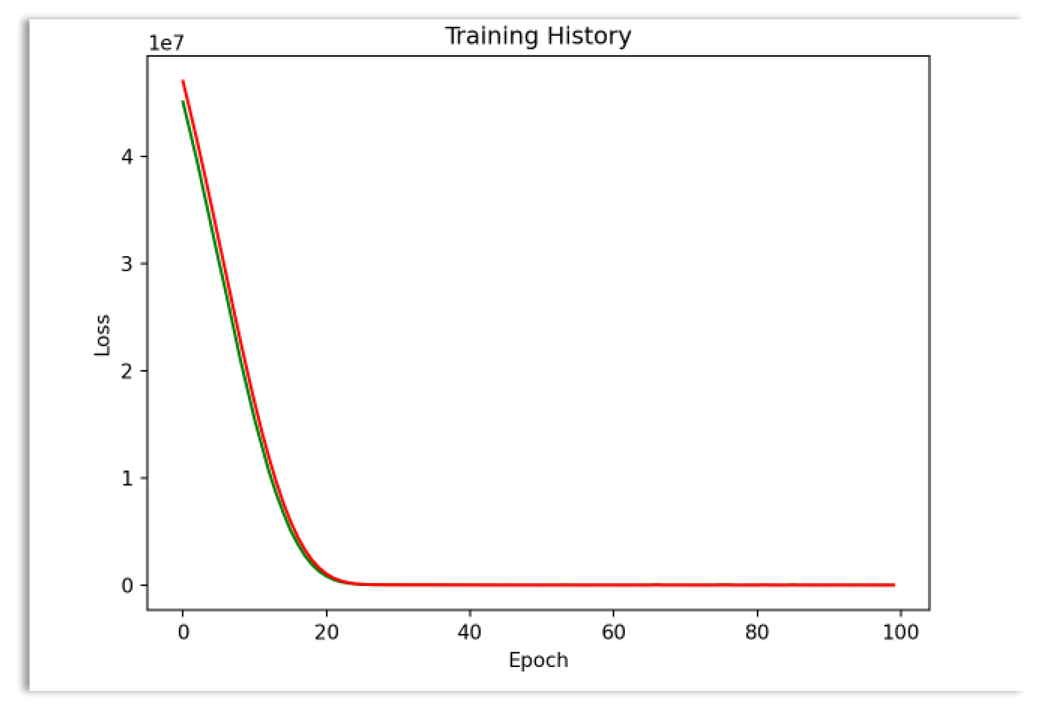 This graph shows that it would be optimal to set the number of epochs to 20.