Lesson 4: Deep Neural Networks (Concepts)

Introduction to Deep Neural Networks

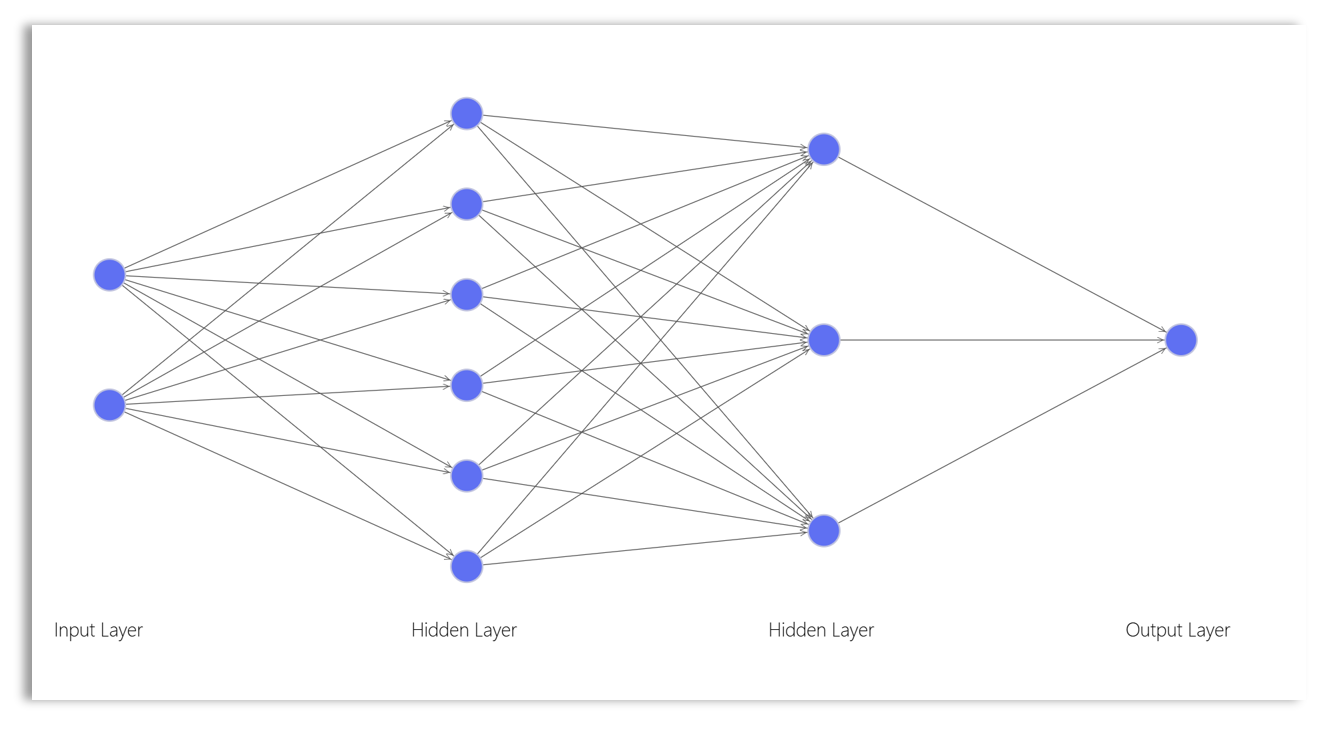
A deep neural network (DNN), also known as an artificial neural network (ANN), is a type of machine learning model composed of multiple layers of data representations. It typically includes an input layer, one or more hidden layers, and an output layer. The input layer receives the initial data, while the output layer produces the final result. The layers between the input and output layers are known as hidden layers.

A neural network is considered “deep” when it has multiple hidden layers. These layers are densely connected to each other, meaning each neuron in one layer is connected to all neurons in the subsequent layer. Each successive layer represents increasingly abstract or latent features of the data.

The Perceptron

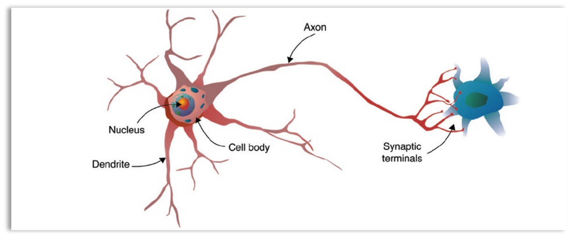
Neural Networks (NN) are designed to emulate or mimic the structure and function of the human brain. In the human brain, a neuron (cell) receives signals from other neurons through its dendrites, processes those signals in its cell body, and transmits the result via its axon to other neurons. Similarly, the computational unit of a Deep Neural Network (DNN), called a perceptron, node, or neuron, receives input from other neurons, processes it using a mathematical function, and sends the output to other neurons in the network.

A diagram of a biological neuron in the human brain.

A diagram of a DNN perception

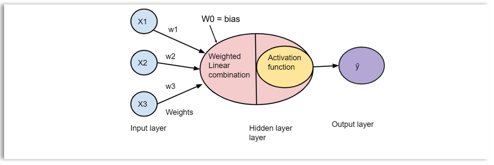
Generally, a perception is a computational unit that transforms inputs into an output, which is a linear combination of inputs. The output is further through an activation (non-linear) function into another output.

A Simple Neural Network Architecture

We will use a simple neural network to explore the different components of a neural network and how they are trained.

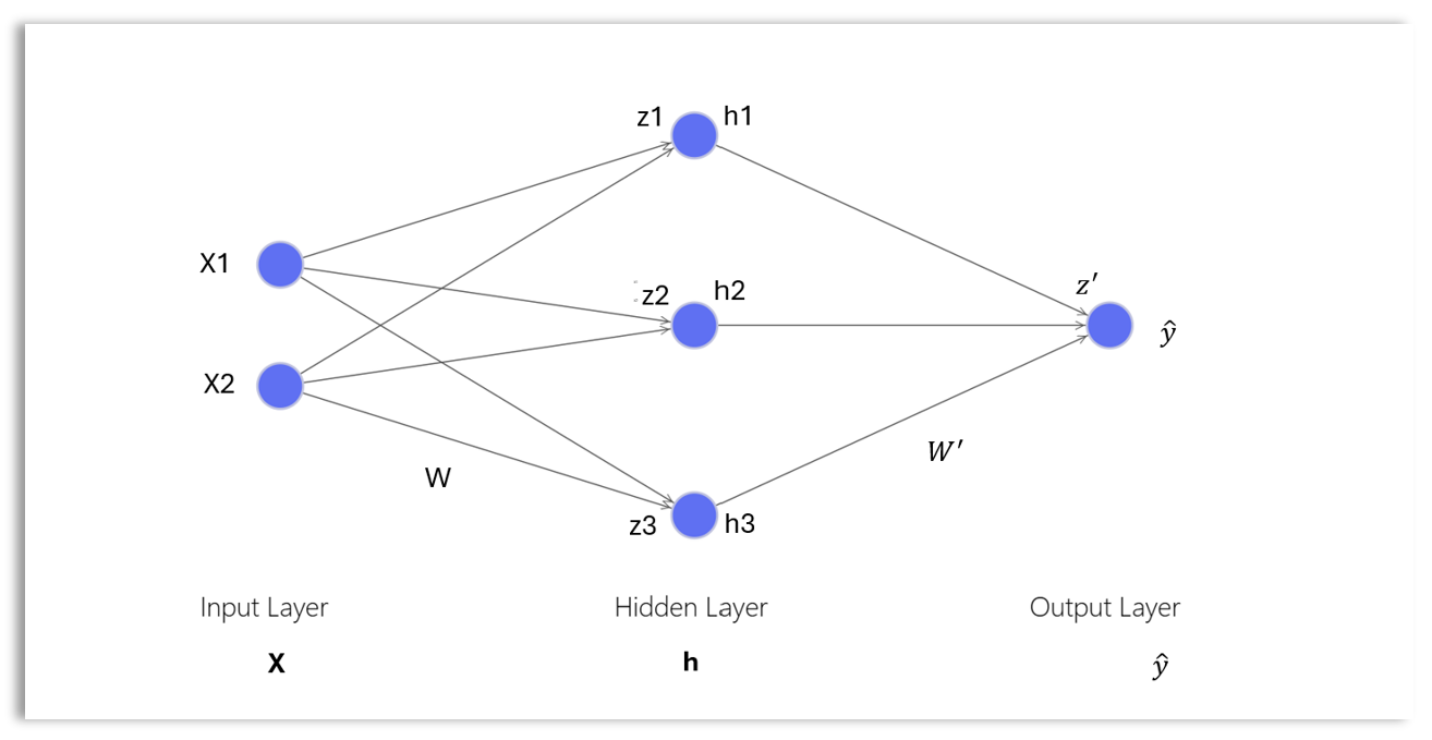
The simple neural network above consists of the following setup:

• Input layer with two nodes: \(x_1\) and \(x_2\)
• Hidden layer with three nodes: \(h_1\), \(h_2\), and \(h_3\)
• Output layer with one node: \(\hat y\)

Input Layer

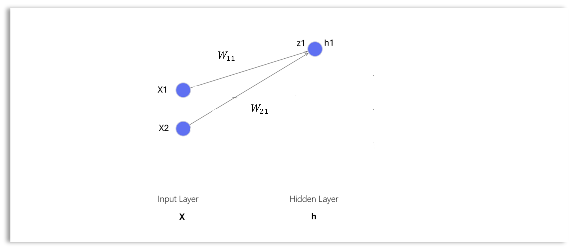
The input layer of a neural network (NN) is the first layer that receives input data, represented as an input vector. The input layer serves as the entry point for the data to enter the network.

The input vector, \(\mathbf{x}\) in the input layer has dimension \(1 \times d_x\), where \(d_x\) is the length of the input vector or number of nodes in the input layer. The input vector of the input layer is written as:

\[ \mathbf{x} = \begin{bmatrix} x_{1} & x_{2} \end{bmatrix} \] where:

• \(\mathbf{x}\) is \(1 \times 2\) row vector representing a single record in the data.
• \(x_1\) and \(x_2\) are the values of the individual features or attributes for a single record or example.

Hidden Layer

The hidden layer is the layer between the input and output layers. A simple neural network has one hidden layer while a deep neural network has several hidden layers.

The weight matrix for the hidden layer: The nodes between layers are connected by weights, which are the parameters of the network, typically represented as a weight matrix, \(W\), with dimension \(d_x \times d_h\).

• \(d_x\) is the length of the input vector or number of nodes in the input layer.
• \(d_h\) is the length of the hidden vector or number of nodes in the hidden layer.

In a simple neural network with two nodes in the input layer and three nodes in the hidden layer, The weight matrix for the hidden layer, \(W\) with dimensions \(2 \times 3\) can be written as:

\[ W = \begin{bmatrix} w_{11} & w_{12} & w_{13} \\ w_{21} & w_{22} & w_{23} \end{bmatrix} \]

In code, this matrix can be written as an array:

\[ W = \begin{matrix} [[w_{11} & w_{12} & w_{13}], \\ w_{21} & w_{22} & w_{23}]] \end{matrix} \] Where:

• \(w_{11}\) is the weight that connects the input \(x_{1}\) to the second hidden neuron \(h_{1}\)
• \(w_{12}\) is the weight that connects the input \(x_{1}\) to the second hidden neuron \(h_{2}\)
• and so on.

The bias vector for the hidden layer: Each layer, except the input layer, has a bias vector (containing bias terms). The biases are additional parameters in the neural network that allow the model to adapt and learn more complex functions or patterns.

The a hidden layer bias term is added to the weighted sum of inputs in each hidden node. The dimension of the bias vector is \(1 \times d_h\), where \(d_h\) is the number of nodes in the hidden layer. Let’s denote the bias vector for the hidden layer as:

\[ \mathbf{b} = \begin{bmatrix} b_{1} & b_{2} & b_{3} \end{bmatrix} \]

Where:

• The dimension of the bias vector for the simple neural network is \(1 \times 3\).
• \({b_1}\), \({b_2}\), and \({b_3}\) are the bias terms for the first, second and third hidden nodes.

Weighted sum of inputs for the hidden layer: The hidden layer consists of nodes that use the weights in the weight matrix,\(W\) to transform the input vector into weighted scores, while incorporating the bias term. The hidden layer first computes the weighted score vector \(\mathbf{z}\), containing weighted sum of inputs plus the bias terms:

\[ \begin{aligned} \mathbf{z} &= \mathbf{x} \mathbf{W} + \mathbf{b} \\ &= \begin{bmatrix} z_1 & z_2 & z_3 \end{bmatrix} \end{aligned} \]

The diagram below shows how the input values are connected to a hidden node through the weights.

The weighted scores at various hidden nodes are calculated as follows:

\[ \begin{aligned} z_1 &= x_1 * w_{11} + x_2 * w_{21} + b1 \\ z_2 &= x_1 * w_{12} + x_2 * w_{22} + b2 \\ z_3 &= x_1 * w_{13} + x_2 * w_{23} + b3 \end{aligned} \]

Output of the hidden layer: The weighted score vector is then processed through an activation function \(f\) (e.g., sigmoid or ReLU) to generate the final hidden layer output vector, \(h\).

\[ \begin{aligned} h & = f(z) \\ &= \begin{bmatrix} h_1 & h_2 & h_3 \end{bmatrix} \end{aligned} \] Where:

\[ \begin{aligned} h_1 &= f(z_1) \\ h_2 &= f(z_2) \\ h_3 &= f(z_3) \end{aligned} \]

The Output Layer

The output layer is the final layer of a neural network. The output layer produces the final prediction of the network, based on the processed data from the previous layers.

The weight matrix \(\mathbf{W'}\) for the output layer has dimensions \(d_h \times 1\), where \(d_h\) is the number of nodes in the hidden layer (assuming a single output node for simplicity):

\[ \mathbf{W'} = \begin{bmatrix} w_1' \\ w_2' \\ w_3' \end{bmatrix} \]

The bias term \(b'\) for the output layer is a scalar.

The weighted sum of inputs for the output layer \(z'\) is computed as:

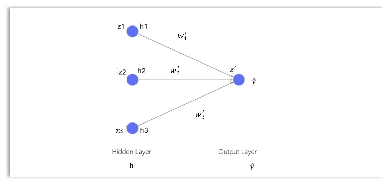
\[ \begin{aligned} z' &= h \cdot \mathbf{W'} + b' \\ &= h_1 \cdot w'_1 + h_2 \cdot w'_2 + h_3 \cdot w'_3 + b' \end{aligned} \]

The final output of the network \(\hat{y}\) depends on the type of problem:

• For Regression: There is no activation function and the output is the weighted score (scalar) \(z'\):

  \[ \hat{y} = z' \]

• For Binary Classification: A sigmoid activation function is applied to obtain the probability of the input belonging to class 1 :

\[ \hat{y} = \text{sigmoid}(z') = \frac{1}{1 + e^{-z'}} \]

• For Multi-class Classification: The softmax activation function is applied to the vector of weighted scores \(z'\) to obtain a vector of probabilities:

\[ \hat{y} = \text{softmax}(z') = \begin{bmatrix} \hat{y}_1 & \hat{y}_2 & \dots & \hat{y}_k \end{bmatrix} \] Where:

\[ \hat{y}_i = \frac{e^{z_i'}}{\sum_{j=1}^{k} e^{z_j'}} \] Each element \(\hat{y}_i\) of the output vector \(\hat{y}\) represents the probability of the input belonging to class \(i\). The sum of all probabilities is 1.

Training a Neural Networks

A neural network is trained through the follow four steps:

Step 1: Initialization

The first step to training a neural network is to set the initial values of weights and biases that allow the network to learn effectively, avoiding issues like vanishing or exploding gradients. Common strategies include initializing weights randomly from a Gaussian or uniform distribution with a small standard deviation.

Step 2: Forward Propagation

In this first step, the input data \(\mathbf{x}\) is passed through the network from the input layer to the output layer. This is known as forward propagation. As the data flows through each layer, it is transformed by applying a series of operations such as weighted sums and activation functions. In the final layer, the network produces a prediction, denoted as \(\hat{y}\), which is the model’s output for the given input.

Step 3: Backpropagation

Backpropagation is basically the process of updating the weights of the neural networks model until the model converges. Backpropagation is implemented through the gradient descent rule: There are different flavors of gradient descent including stochastic gradient descent, RMSprop, Adam, Adadelta, Adagrad, Adamax, Nadam, etc. Here is a typical gradient descent rule for updating the weights:

\[ w := w - \alpha \cdot \frac{\partial J(w, b)}{\partial w} \] To update each weight, we need to compute the gradient or the derivative of the loss function with respect to that weight and use that gradient in the gradient descent rule (optimizer).

Computing the Gradient of Weights in a Neural Networks

Let’s first revisit how to compute gradient of the loss function for a linear regression and logistic regression.

• For a regression problem, we can use the MSE loss function expressed as:

  \[ J(w, b) = \frac{1}{2m} \sum_{i=1}^{m} (y_i - \hat{y}_i)^2 \]

  and for a linear regression model (perceptron without a non-linear activation function):

  \[ \frac{\partial J(w, b)}{\partial w} = \frac{1}{m} \sum_{i=1}^{m} ( \hat{y}_i - y_i ) \cdot x_i \]

• For a binary classification problem, we can use the cross-entropy loss function expressed as:

  \[ J(w, b) = -\frac{1}{m} \sum_{i=1}^{m} \left[ y_i \log(\hat{y}_i) + (1 - y_i) \log(1 - \hat{y}_i) \right] \]

  For a logistic regression model (perceptron):

  \[ \frac{\partial J(w, b)}{\partial w} = \frac{1}{m} \sum_{i=1}^{m} \left( \hat{y}_i - y_i \right) \cdot x_i \]

It is easy to compute the gradient for linear regression and logistic regression models as shown above. However, for more complex neural networks, the gradient of the cost function with respect to a parameter is computed using the chain rule, as illustrated in the diagram below.

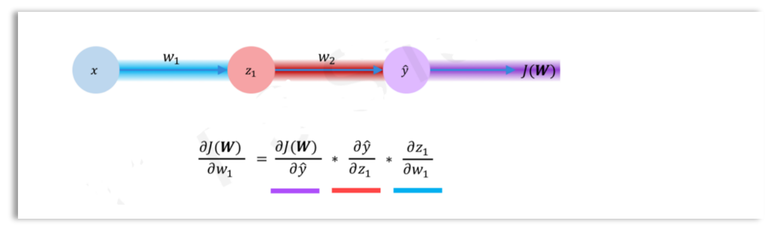
Chain Rule for Gradient of Weights \(w_1\)

We want to compute the gradient of the loss \(J\) with respect to the weight \(w_1\) for a single path in a neural network with one hidden layer.

The chain rule for \(\frac{dJ}{dw_1}\) for a single path is computed as:

\[ \frac{dJ}{dw_1} = \frac{dJ}{d\hat{y}} \cdot \frac{d\hat{y}}{dz_2} \cdot \frac{dz_2}{da_1} \cdot \frac{da_1}{dz_1} \cdot \frac{dz_1}{dw_1} \]

Where:

• \(\hat{y}\) is the output of the network (the predicted value).
• \(z_2 = w_2 a_1 + b_2\) is the linear combination for the output layer.
• \(a_1\) is the output of the hidden layer after applying the activation function.
• \(z_1 = w_1 x + b_1\) is the linear combination for the hidden layer, where \(x\) is the input feature vector.

Now, let’s break down each term in the chain rule:

1. Loss Gradient w.r.t. Output (\(\hat{y}\)):

   For binary cross-entropy loss: \[ \frac{dJ}{d\hat{y}} = \frac{\hat{y} - y}{\hat{y}(1 - \hat{y})} \]

2. Derivative of Activation (Sigmoid) w.r.t. \(z_2\): \[ \frac{d\hat{y}}{dz_2} = \hat{y}(1 - \hat{y}) \]

3. Derivative of \(z_2\) w.r.t. \(a_1\): \[ \frac{dz_2}{da_1} = w_2 \]

4. Derivative of Activation (Sigmoid) w.r.t. \(z_1\): \[ \frac{da_1}{dz_1} = a_1(1 - a_1) \]

5. Derivative of \(z_1\) w.r.t. \(w_1\): \[ \frac{dz_1}{dw_1} = x \]

Now, combining all of the above terms, we get:

\[ \frac{dJ}{dw_1} = (\hat{y} - y) \cdot w_2 \cdot a_1(1 - a_1) \cdot x \]

Thus, the gradient of the loss function with respect to the weight \(w_1\) is:

\[ \frac{dJ}{dw_1} = (\hat{y} - y) \cdot w_2 \cdot a_1(1 - a_1) \cdot x \]

Note

If there are several paths that lead to a parameter, the total derivative of the loss with respect to that parameter is the sum of the gradients contributed by each path.

Types of Activation Functions

Activation functions are squashing functions that map real values to values within a smaller range. The purpose of activation functions is to introduce non-linearity in the neural network. Non-linear activation functions allow us to learn more complex non-linear decision boundaries, which is especially useful for classification problems.

There are different types of activation functions, including:

• Sigmoid function: The sigmoid (logistic) function outputs values between 0 and 1. This is a good choice for the output layer in a binary classification problem since these values can be interpreted as the probability of an input belonging to the desired class (class 1).

• Tanh function: The output of the \(tanh\) function is always between -1 and 1. This makes \(tanh\) a better choice for hidden layers since it keeps the average of the outputs in each layer close to zero.

• ReLU function: \(g(z) = \max(0, z)\). ReLU is also a good choice for hidden layers and is preferred over \(tanh\) because it speeds up the learning process. This is due to the fact that its derivative is easier to compute. The derivative is 1 when \(z > 0\) and \(0\) when \(z \leq 0\).

• Softmax: Softmax is a generalization of the logistic function to multiclass classification problems. It is used in multiclass logistic regression and specified as the activation function in a neural network for classification problems with more than two classes. The softmax function takes a vector \(z\) of \(k\) values and transforms them into a vector of \(k\) probabilities. It is commonly used in the output layer of a neural network for multiclass classification problems.

Summary

This lesson introduces the concept of Deep Neural Networks (DNNs), a type of machine learning model designed to emulate the human brain. DNNs are composed of multiple layers, including an input layer, one or more hidden layers, and an output layer. These layers are densely connected, with each neuron in one layer being linked to all neurons in the next. The key to a DNN’s “depth” lies in its multiple hidden layers, which allow it to progressively learn more abstract features from the data. The lesson also explains the perceptron, the computational unit of a neural network, which processes inputs using mathematical functions and produces outputs that can be passed to subsequent neurons.

The lesson goes on to explore the architecture of a simple neural network, detailing the input layer, hidden layer, and output layer. It illustrates how data flows through the network, starting with the input layer and passing through weighted connections and bias terms in the hidden layer, followed by an activation function. The output layer generates predictions based on the processed data.

The process of training a neural network is explained step-by-step, including initialization, forward propagation, and backpropagation. Backpropagation is critical for adjusting the network’s weights using gradient descent, helping the model converge on optimal parameters. Additionally, the lesson introduces various activation functions (like sigmoid, tanh, and ReLU) and their roles in enabling the network to learn complex patterns and make predictions for different types of problems, such as binary or multi-class classification.