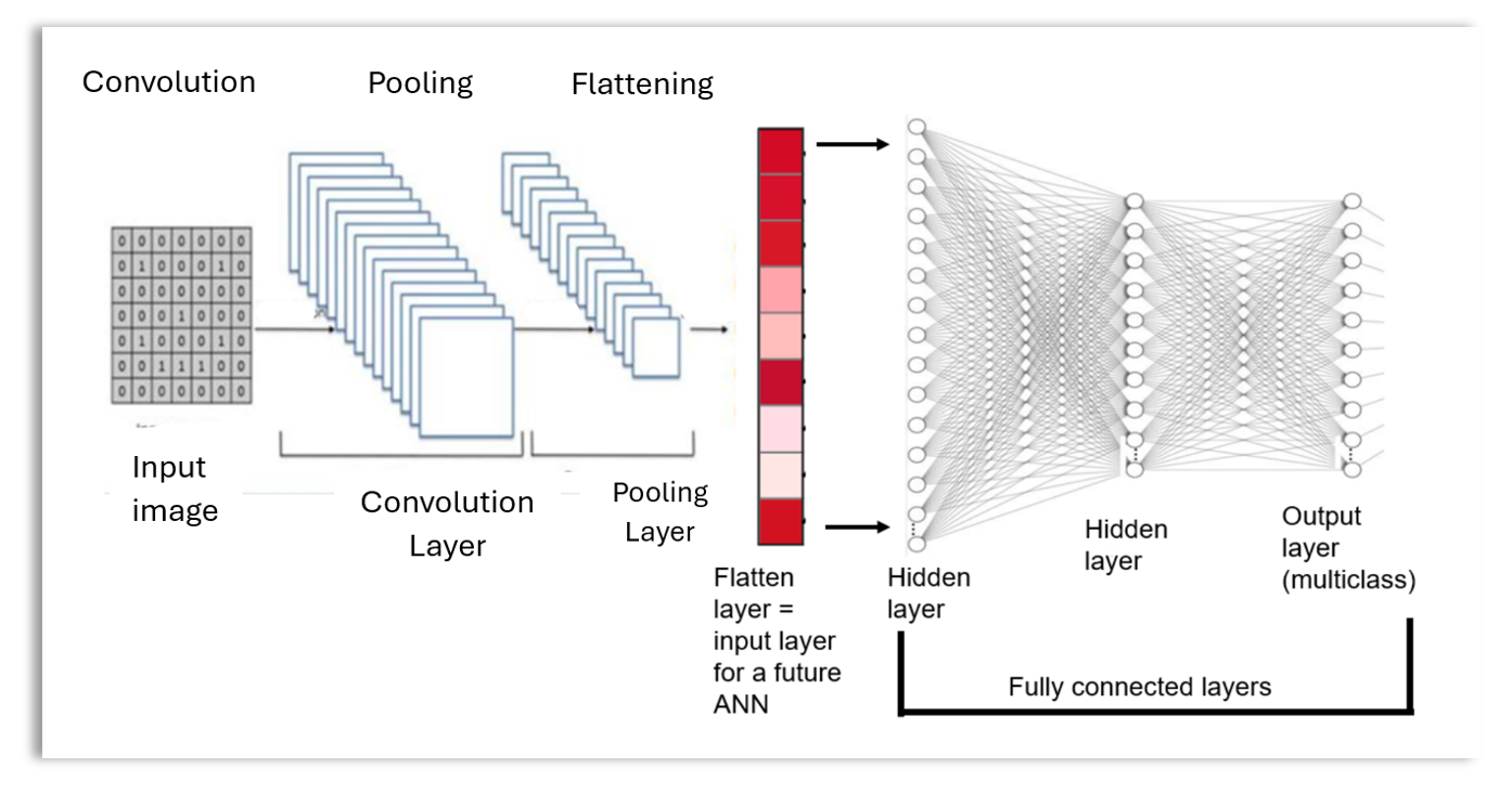
A convolutional neural network (CNN) is a special type of neural network where feature extraction is performed through convolutional and pooling layers before the transformed data is passed to the fully connected layers. This means the convolutional neural network architecture consists of the input layer, a series of convolutional and pooling layers, a flattening layer, and fully connected layers.
As shown in the convolutional neural network diagram above, the first layer is the input layer. Between the input layer and the flattening layer, there is a series of convolutional and pooling layers used for feature extraction.
Why do we Need a Convolutional Neural Network?
When working with a color image dataset, we could unpack the dataset into a 2D format as a preprocessing step before using the data for modeling. However, this can be problematic when the color image dataset is large. Unpacking a large color image dataset into a 2D format can greatly increase the number of “features” or parameters, potentially leading to overfitting.
For example, the CIFAR-10 training dataset consists of 50,000 32x32 color images with shape (50000, 32, 32, 3). If we unpack this dataset into a 2D format, it will have a shape of (50000, 3072). If we were using this 2D dataset for a single perceptron, there would be 3072 weights. The number of weights increases further if there are hidden layers with multiple units or if the image dimensions are larger.
Therefore, it is beneficial to extract relevant features before passing the data to the fully connected layers for processing. Convolutional neural networks provide an excellent way to automatically perform feature extraction through their convolutional and pooling layers.
Convolutional Neural Network Operations
The process of building a convolutional neural network involves four major steps: 1) Convolution, 2) Pooling, 3) Flattening, and 4) Fully connected layers.The first part of the CNN (before the fully connected layers) is called the convolutional base, while the second part (the fully connected layers only) of the CNN is called the classifier. Let’s now discuss the key operations, such as convolution and pooling, involved in building a convolutional neural network model.
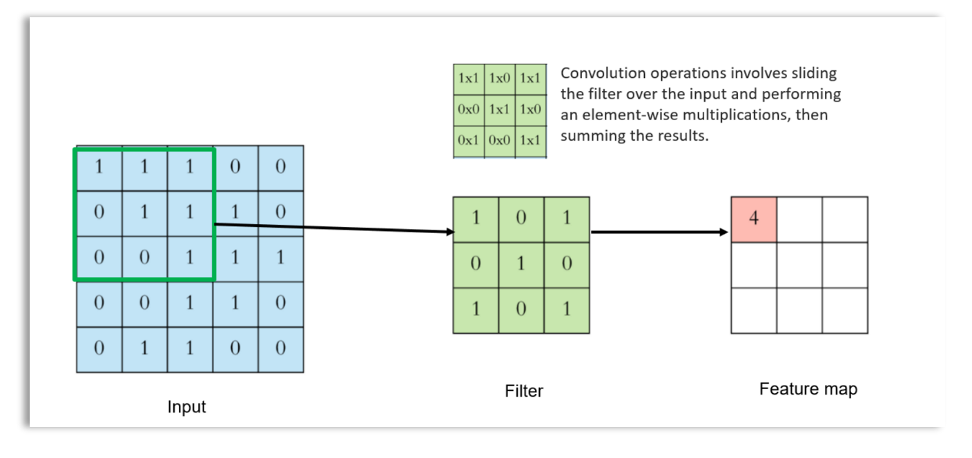
The Convolution Operation
The convolution operation is performed in the convolutional layer. It involves transforming the input data into a feature map using a convolution filter (also called a kernel or detector). Here is an example of a convolution operation with 2D input data and a 3x3 filter.
Color images are usually 3D (RGB), so a 3D filter is needed when the image is 3D. For example, when working with a 3D image, we could slide a 5x5x3 filter across a 32x32x3 color image. When the filter is positioned in a particular region, it covers a small volume of the input, where the convolution operation will be performed. The matrix multiplication is done in 3D, and all the results are summed to obtain a single value. As we scan through the entire image, a 2D output is produced.
Different filters are used to capture or extract various aspects of the image. So, if 12 filters are used, there will be 12 2D outputs stacked together to form a 3D volume output, as shown below:
The resulting output from 12 filters will have a volume of 32x32x12. An activation function can be applied to scale the output volume, which will change the values of the output, but the volume will remain the same, 32x32x12. The feature map obtained from the convolutional layer is then passed to the pooling layer for further processing.
The Hyper Parameters of the filter
Filter Dimension: The size of the filter, such as 3x3, 5x5, or 7x7, is a hyperparameter that can be optimized. The depth of the filter usually corresponds to the depth of the image, so we typically leave that out.
Number of Filters (Depth of the Output Volume): The number of filters used is an important hyperparameter that can be tuned.
Strides: Strides refer to the number of pixel shifts over the input data after each convolution operation. The default value is 1, meaning the filter shifts by one pixel after each operation. Note that strides can also be a hyperparameter when pooling is applied. Therefore, strides are a hyperparameter for both convolution and pooling layers.
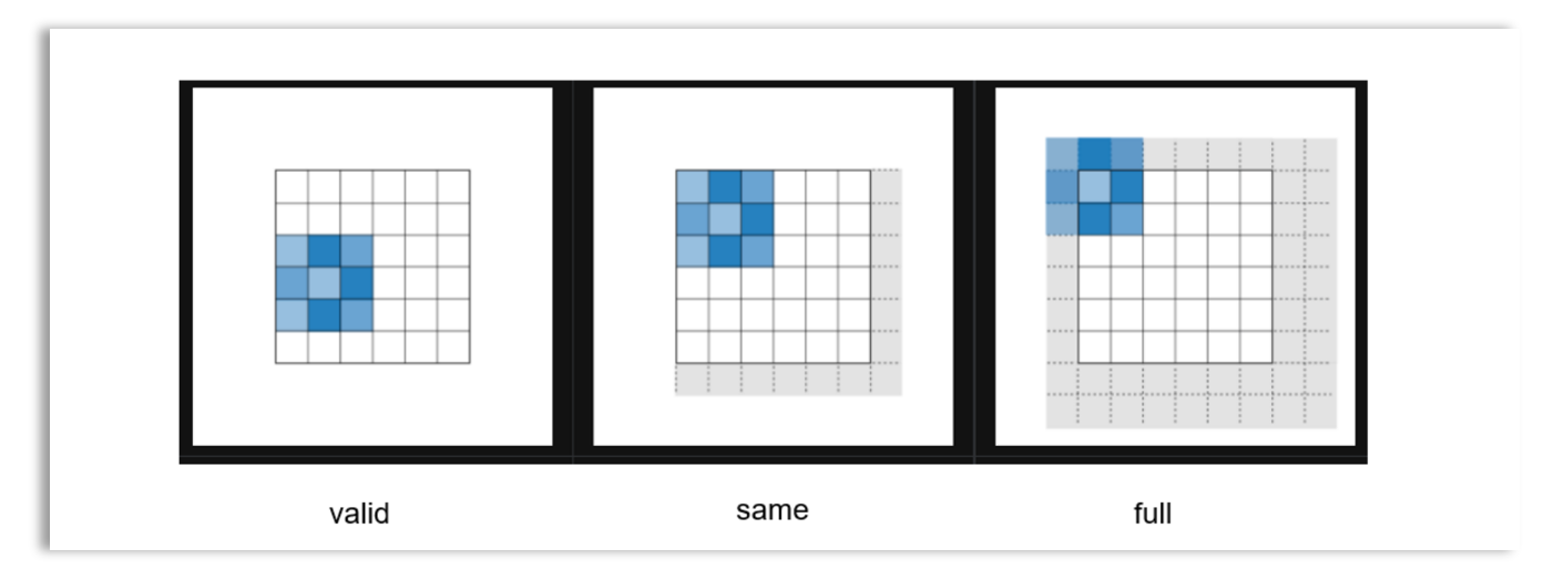
Padding: As we scan the input data with the filter, the filter may not always fit perfectly. To address this, we can use zero-padding, where zeros are added around the borders of the image, or we can drop the part of the image where the filter does not fit. There are different modes of zero-padding, as shown below:
Valid: In this mode, no padding is applied. The convolution is performed only on the regions where the filter fully fits. Parts of the input that do not match are excluded.
Same: In this mode, padding is applied so that if strides = 1, the feature map has the same size as the input data. If strides = 2, the feature map is half the size of the input data. This is why “same padding” is also called “half padding.”
Full: This mode applies maximum padding, allowing the convolution to be performed even at the boundaries of the input.
Padding helps control the height and width of the output volume. The most commonly used padding is “same” padding, as it preserves the spatial size of the input by ensuring that the height and width of the input and output volumes are the same.
The Pooling Operation
The pooling operation is a type of “dimensionality reduction” or downsampling technique achieved by sliding a pooling window across a 3D input. The pooling layer helps us ignore less important features in the image and further reduce the image size, while preserving important features. For example, if we have a picture of a cat sitting on a carpet, pooling helps extract the features of the cat and ignore the carpet.
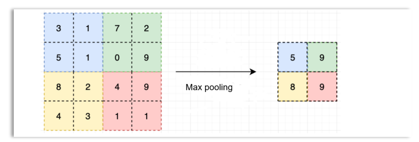
There are three main types of pooling operations: max pooling, min pooling, and average pooling, where the maximum, minimum, or average of the values in the region of the input data covered by the fixed-size pooling window is used as the output. Pooling only reduces the height and width of the input data, but the depth remains the same. For example, a pooling window of size 4x4 could be used to transform a 32x32x3 input into a 16x16x3 output.
Here is an example of max pooling, where a 2x2 window is used to transform a 4x4 image into a 2x2 output.
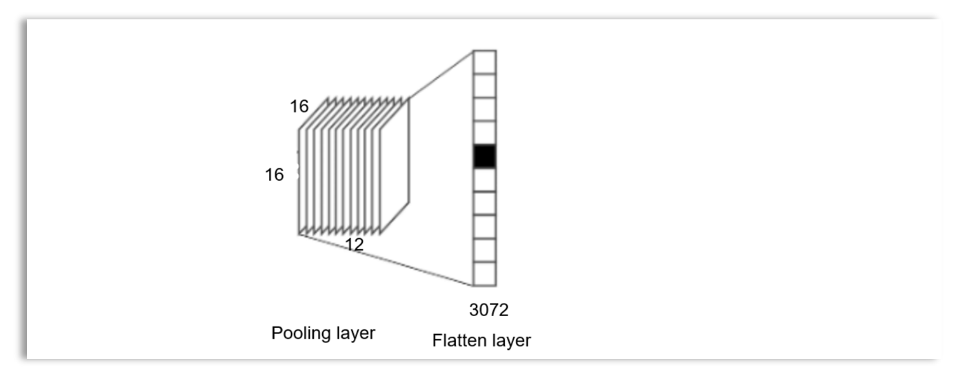
Flattening
For each image, flattening unpacks the pooled output volume into a vector of data, which can then be processed through the fully connected layers of the artificial neural network. The output of the flattening layer serves as the input to the artificial neural network. If flattening is applied to an output with a volume of 16x16x12 from the pooling layer, a vector of 3072 values will be obtained, as shown below:
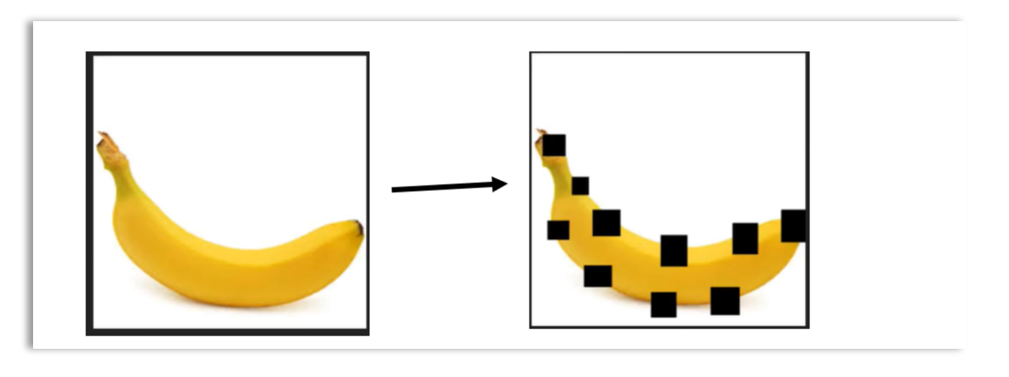
Dropout Operation
Dropout involves randomly setting certain portions of the input (e.g., image pixels) to zero during training. This technique helps build a model that generalizes well to unseen examples.
No parameters are learned in the dropout layer. In Keras, the dropout layer can be defined by specifying the percentage of neurons (or pixels) that should be dropped or set to zero.
Below is an illustration of dropout:
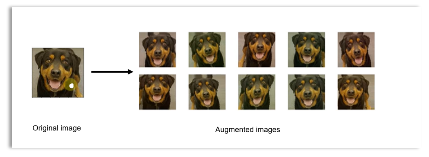
Image Augumentation
Image augmentation involves applying random transformations to each image, such as rotations, shifting, flipping, and more. These transformations are applied during each epoch, so each epoch uses a different variant of the original image. As a result, it appears as though the dataset has been increased due to the different variants of the images used in each epoch.
Image augmentation is a preprocessing step used to generate more images from existing ones. This helps create more representative data that can generalize well to unseen test samples, thereby preventing overfitting.
Image augmentation helps us train models that are more robust and have better accuracy, as the models are exposed to different variations of the same image. Color shifting is another technique used for image augmentation, where different RGB values are applied to distort the color channels. Random cropping is also a technique used for image augmentation.
A Convolutional Neural Network for Image Classification
We will use the CIFAR-10 image dataset in Keras to illustrate how to construct a convolutional neural network model. The architecture of the convolutional neural network will consists of the following layers:
NoteCNN Architecture
Input layer
Convolutional layer + ReLU
Pooling layer
Convolutional layer + ReLU
Pooling layer
Flatten layer
Fully connected layer
Hidden layer + ReLU
Hidden layer + ReLU
Output layer + Softmax
Preprocessing of Image Data
Code
from keras.datasets import cifar10import keras# Load CIFAR-10 data(x_train_ci, y_train_ci), (x_test_ci, y_test_ci) = cifar10.load_data()# Scale the input data (normalize to range [0, 1])x_train_ci = x_train_ci /255x_test_ci = x_test_ci /255# Transform output data to categorical (one-hot encoded)y_train_ci = keras.utils.to_categorical(y_train_ci)y_test_ci = keras.utils.to_categorical(y_test_ci)print(f"Training data shape: {x_train_ci.shape}, {y_train_ci.shape}\n"f"Test data shape: {x_test_ci.shape}, {y_test_ci.shape}")
Training data shape: (50000, 32, 32, 3), (50000, 10)
Test data shape: (10000, 32, 32, 3), (10000, 10)
Build the CNN Model
Code
import tensorflow as tfimport kerasfrom keras import layers# Set random seed for reproducibilitytf.random.set_seed(1234)# Initialize the Sequential modelmodel = keras.Sequential()# Use the Input layer to specify the input shapemodel.add(layers.Input(shape=(32, 32, 3))) # Specify the input shape# First convolutional layer with 28 filters of size (3x3), ReLU activation, and 'same' paddingmodel.add(layers.Conv2D(28, (3, 3), activation='relu', padding='same'))# Max pooling layer with a pool size of (2x2)model.add(layers.MaxPooling2D((2, 2)))# Second convolutional layer with 64 filters of size (3x3) and ReLU activationmodel.add(layers.Conv2D(64, (3, 3), activation='relu'))# Max pooling layer with a pool size of (2x2)model.add(layers.MaxPooling2D((2, 2)))# Flatten the output to feed into fully connected layersmodel.add(layers.Flatten())# Fully connected layer with 512 units and ReLU activationmodel.add(layers.Dense(512, activation='relu'))# Output layer with 10 units (for 10 classes) and softmax activationmodel.add(layers.Dense(10, activation='softmax'))# Compile the model with RMSprop optimizer, categorical crossentropy loss, and accuracy metricmodel.compile(optimizer='rmsprop', loss='categorical_crossentropy', metrics=['accuracy'])# Train the model on the training data for 8 epochs with a batch size of 128model.fit(x_train_ci, y_train_ci, epochs=8, batch_size=128, verbose=0)
<keras.src.callbacks.history.History object at 0x7fd247d9c250>
# Evaluate the modeltrain_acc = model.evaluate(x_train_ci, y_train_ci, verbose=0)[1]test_acc = model.evaluate(x_test_ci, y_test_ci, verbose=0)[1]# Print the accuracy on training and test setsprint(f"Accuracy on Training Set: {train_acc}")
Accuracy on Training Set: 0.8812400102615356
Code
print(f"Accuracy on Test Set: {test_acc}")
Accuracy on Test Set: 0.7028999924659729
Add a Dropout Layer
We could add a dropout layer after the flatten layer using the code: model.add(layers.Dropout(0.5)).
Specifying 0.5 in the dropout layer implies we want to drop 50% of the pixels in each image, not 5%. Dropout improves the model by reducing overfitting.
Code
import tensorflow as tffrom tensorflow import kerasfrom tensorflow.keras import layers# Set random seed for reproducibilitytf.random.set_seed(1234)# Build the model with dropout layermodel = keras.Sequential()# Use the Input layer to specify the input shapemodel.add(layers.Input(shape=(32, 32, 3))) # Add the first convolutional layer with 28 filters and (3x3) kernel sizemodel.add(layers.Conv2D(28, (3, 3), activation='relu', padding='same'))# Add max pooling layer with (2x2) pool sizemodel.add(layers.MaxPooling2D((2, 2)))# Add the second convolutional layer with 64 filters and (3x3) kernel sizemodel.add(layers.Conv2D(64, (3, 3), activation='relu'))# Add another max pooling layer with (2x2) pool sizemodel.add(layers.MaxPooling2D((2, 2)))# Flatten the output to pass it to fully connected layersmodel.add(layers.Flatten())# Add dropout layer to reduce overfitting, dropping 50% of the pixelsmodel.add(layers.Dropout(0.5))# Add fully connected layer with 512 units and ReLU activationmodel.add(layers.Dense(512, activation='relu'))# Add the output layer with 10 units and softmax activation (for 10 classes)model.add(layers.Dense(10, activation='softmax'))# Compile the model with RMSprop optimizer, categorical crossentropy loss, and accuracy metricmodel.compile(optimizer='rmsprop', loss='categorical_crossentropy', metrics=['accuracy'])# Train the model on the training data for 8 epochs with a batch size of 128model.fit(x_train_ci, y_train_ci, epochs=8, batch_size=128, verbose=0)
<keras.src.callbacks.history.History object at 0x7fd1ade82ed0>
After the adding a dropout layer, the performance of the model is as follows:
Code
# Evaluate the model on the training and test datatrain_acc = model.evaluate(x_train_ci, y_train_ci, verbose=0)[1]test_acc = model.evaluate(x_test_ci, y_test_ci, verbose=0)[1]# Print the accuracy resultsprint(f"Accuracy on Training Set: {train_acc}\nAccuracy on Test Set: {test_acc}")
Accuracy on Training Set: 0.8166800141334534
Accuracy on Test Set: 0.7174000144004822
Summary
The lesson on Convolutional Neural Networks (CNNs) focuses on understanding how CNNs are structured and their operations, which make them effective for image classification tasks. CNNs are composed of layers that perform convolution, pooling, flattening, and finally, fully connected operations. Convolutional layers apply filters to the input image, producing feature maps, which are further processed by pooling layers to reduce dimensionality while preserving key features. The flattened output is passed to fully connected layers for classification, making CNNs highly efficient in handling image data by automatically performing feature extraction. Additionally, hyperparameters such as filter size, number of filters, and padding types (e.g., ‘valid’, ‘same’, ‘full’) can be optimized to improve model performance. CNNs provide significant advantages over traditional models in terms of processing large datasets efficiently.
The lesson also explores key techniques like dropout and image augmentation, which improve the robustness and performance of CNN models. Dropout layers help mitigate overfitting by randomly deactivating a certain percentage of neurons during training, thus promoting better generalization. Image augmentation, which involves applying random transformations to images, further aids in preventing overfitting by artificially expanding the dataset. The lesson demonstrates how to build and train a CNN using the CIFAR-10 dataset in Keras, including the addition of dropout layers to improve model accuracy.
 Color images are usually 3D (RGB), so a 3D filter is needed when the image is 3D. For example, when working with a 3D image, we could slide a 5x5x3 filter across a 32x32x3 color image. When the filter is positioned in a particular region, it covers a small volume of the input, where the convolution operation will be performed. The matrix multiplication is done in 3D, and all the results are summed to obtain a single value. As we scan through the entire image, a 2D output is produced.
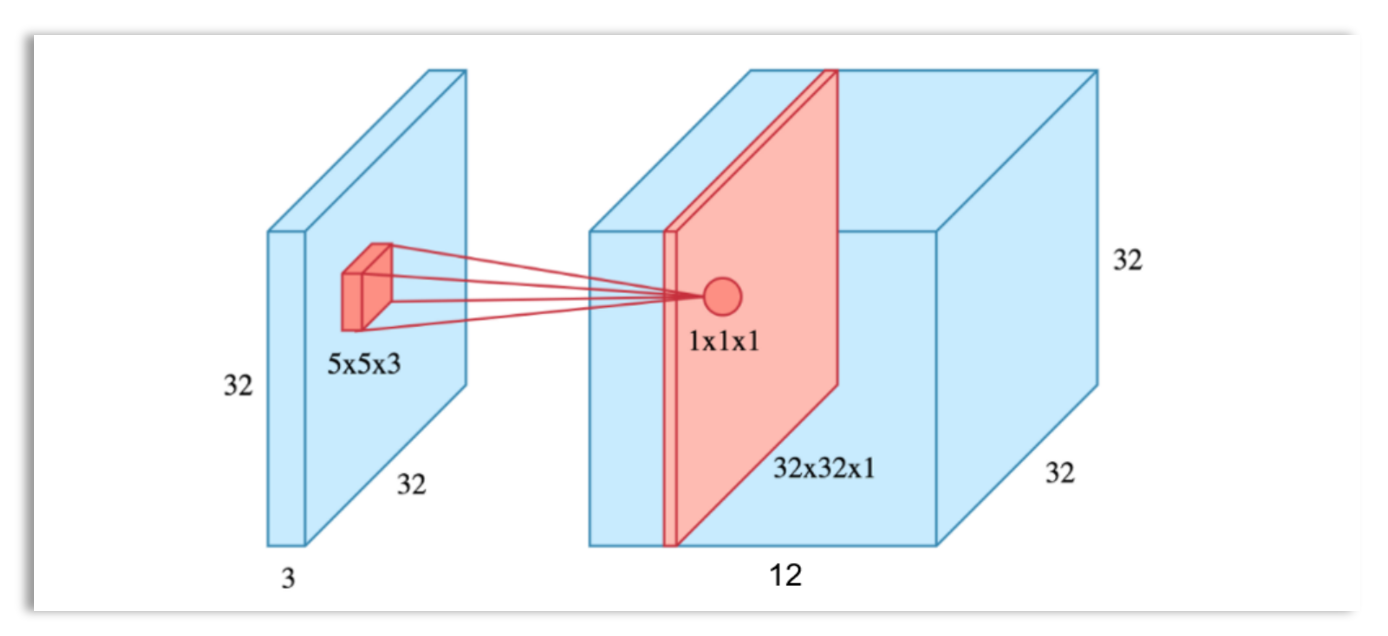 The resulting output from 12 filters will have a volume of 32x32x12. An activation function can be applied to scale the output volume, which will change the values of the output, but the volume will remain the same, 32x32x12. The feature map obtained from the convolutional layer is then passed to the pooling layer for further processing.