In this lesson, we will explore logistic regression, a powerful algorithm used in machine learning for classification tasks. Unlike linear regression, which predicts continuous values, logistic regression estimates the probability that a record belongs to a particular class given the input values. The probability of the record belonging to each class in the target variable is computed, and the record is then classified into the class with the highest probability. The class with the highest probability is the predicted class.We could use logistic regression to predict whether a customer will purchase a product (1) or not (0), based on variables like age, income, or previous purchasing behavior.
A logistic regression model serves three primary purposes:
Probability Estimation: Computing the probability of a given record belonging to a particular class.
Classification: Assigning instances to the class with the highest predicted probability.
Relationship Analysis: Estimating the influence of various independent variables on the dependent variable, providing insights into the relationships within the data.
There are two types of logistic regression:
Binary Logistic Regression: This is a logistic regression model where the outcome is a categorical variable with two possible values or classes.
Multiclass Logistic Regression: This is a logistic regression model where the outcome is a categorical variable with more than two possible values or classes.
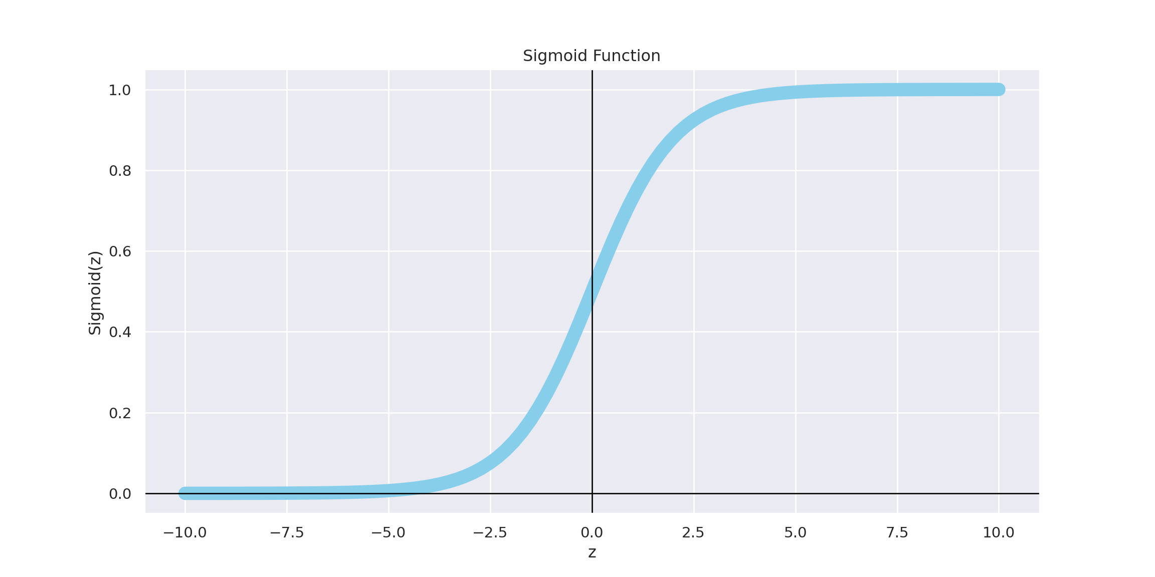
The Logistic Function (Sigmoid Curve)
To understand logistic regression, it’s important to first look at the logistic function, also known as the sigmoid function. The logistic function maps any real-valued number to a value between 0 and 1, which can be interpreted as a probability. This sigmoid function has an S-shaped curve, as shown below:
Code
import numpy as npimport seaborn as snsimport matplotlib.pyplot as plt# Define the sigmoid function using zdef sigmoid(z):return1/ (1+ np.exp(-z))# Create an array of values from -10 to 10 for zz = np.linspace(-10, 10, 100)# Compute the sigmoid of each value in the arrayy = sigmoid(z)# Set the 'darkgrid' style using seaborn (similar to ggplot)sns.set_theme(style="darkgrid")# Plot the sigmoid functionplt.figure(figsize=(12, 6))plt.plot(z, y, label="Sigmoid Function", color="skyblue", linewidth=10)plt.title("Sigmoid Function")plt.xlabel("z")plt.ylabel("Sigmoid(z)")plt.axhline(0, color='black',linewidth=1)plt.axvline(0, color='black',linewidth=1)plt.grid(True)plt.show()
\[
\sigma(z) = \frac{1}{1 + e^{-z}}
\]
Where:
\(z\) is the linear combination of the input variables, i.e.,
\(\sigma(z)\) represents the estimated probability that a record belongs to class 1, given the input variables. Mathematically, this is expressed as \(\sigma(z) = P(y = 1 | X)\).
\(P(y = 1 | X)\) is the estimated probability that a record belongs to class \(y=1\), given the input \(X\),
\(\beta_0\) is the intercept term, and
\(\beta_1, \beta_2, \dots, \beta_n\) are the coefficients of the model that represent the relationship between the input variables and the outcome.
The output of logistic regression is a probability, but if we need a binary classification (0 or 1), we typically apply a threshold. For example, if the predicted probability is greater than 0.5, we classify the outcome as 1; otherwise, it is classified as 0.
From Logistic Function to Log-Odds
The logistic function can be written in the Log-Odds from
\[
P(y=1) = \sigma(z) = \frac{1}{1 + e^{-z}}
\]
The log-odds is the natural logarithm of the odds ratio. The odds ratio is the ratio of the probability of the event occurring to the probability of it not occurring:
This is the key relationship in logistic regression, where the log-odds is modeled as a linear combination of the input features.
Logistic Regression Use Cases
Logistic regression is widely used for classification tasks in various fields:
Email Spam Detection: Classifying emails as “spam” (1) or “not spam” (0) based on features like subject lines, sender, and body content.
Credit Scoring: Predicting whether a loan application will be approved (1) or denied (0) based on variables like income, debt, and credit history.
Medical Diagnosis: Predicting the likelihood of a disease based on medical reports or records (e.g., predicting whether a patient is at risk of diabetes or not).
Relationship Analysis: We can also use the logistic regression model (logit) to understand how a unit increase in GRE score impacts the odds of admission to a top university.
Logistic Regression in Action: Predicting Loan Approval
Let’s simulate a logistic regression scenario where we predict loan approval based on the applicant’s credit score and income.
The Logistic Regression Model
The model for predicting loan approval can be written as:
We’ll generate a synthetic dataset of 100 applicants, with two features: Credit Score and Income, and a binary outcome: whether the loan was approved (1) or denied (0).
Code
import numpy as npimport pandas as pdimport matplotlib.pyplot as pltfrom sklearn.model_selection import train_test_splitfrom sklearn.linear_model import LogisticRegressionfrom sklearn.metrics import confusion_matrix, classification_reportfrom sklearn import metrics# Set random seed for reproducibilitynp.random.seed(12345)# Simulate data for Credit Score, Income, and Loan Approval (1 = Approved, 0 = Denied)## Random credit scores between 300 and 850credit_scores = np.random.uniform(300, 850, 100).round(0) # Random income between $20,000 and $100,000income = np.random.uniform(20000, 100000, 100).round(2) # Generate random choice for binary loan approval outcomes (1 = approved, 0 = denied)loan_approval = np.random.choice([0, 1], size=100, p=[0.40, 0.60])# Create a DataFramedata = pd.DataFrame({'Credit Score': credit_scores, 'Income': income, 'Loan Approval': loan_approval})# Display the first few rowsdata.head().style.format({'Credit Score': '{:.0f}', 'Income': '{:.2f}'})
Credit Score
Income
Loan Approval
0
811
35663.60
1
1
474
43560.11
0
2
401
70159.99
1
3
413
26897.85
1
4
612
31435.60
0
Step 2: Split the Data into Training and Testing Sets
Next, we’ll split the data into training and testing sets to build and evaluate the model.
Code
# Split data into features (X) and target (y)X = data[['Credit Score', 'Income']] # Featuresy = data['Loan Approval'] # Target# Split the data into training and testing sets (80% training, 20% testing)X_train, X_test, y_train, y_test = train_test_split(X, y, test_size=0.4, random_state=40)
Step 3: Fit the Logistic Regression Model
Now we’ll initialize the logistic regression model, train it on the training data, and make predictions on the test set.
Code
# Initialize the Logistic Regression modelmodel = LogisticRegression()# Train the modelmodel.fit(X_train, y_train);# Make predictions on the test sety_pred = model.predict(X_test)# Evaluate the modelconf_matrix = confusion_matrix(y_test, y_pred)class_report = classification_report(y_test, y_pred)print("\nClassification Report:\n", class_report)
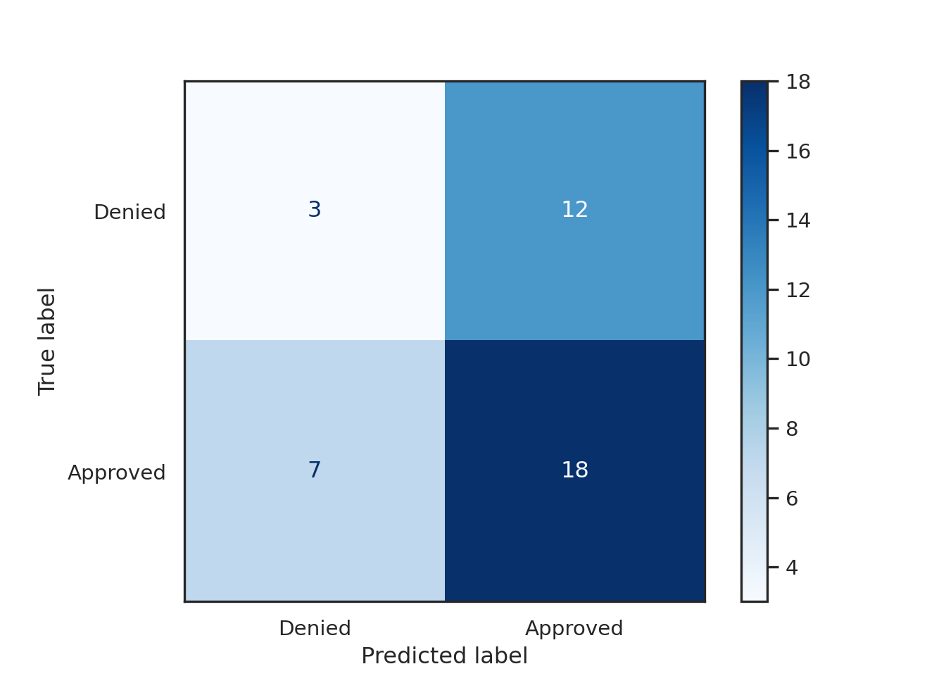
from sklearn.metrics import ConfusionMatrixDisplaysns.set_theme(style="white")# Assuming you already have a fitted model (e.g., knn) and test data (X_test, y_test)cm = confusion_matrix(y_test, model.predict(X_test))# Plot confusion matrix using ConfusionMatrixDisplaydisp = ConfusionMatrixDisplay(confusion_matrix=cm, display_labels=['Denied', 'Approved'])disp.plot(cmap='Blues');
Step 4: Interpret the Results
The Confusion Matrix gives us insight into the number of true positives, true negatives, false positives, and false negatives.
The Classification Report provides performance metrics like accuracy, precision, recall, and F1-score.
The logistic regression model will output the coefficients for each feature, and we can interpret the model as follows:
Intercept\(\beta_0\): The base log-odds of loan approval when both credit score and income are zero.
Coefficients\(\beta_1\), \(\beta_2\): The log-odds change in loan approval for each unit increase in credit score and income. Log-odds are not intuitive so you may exponentiate the coefficients and use those values as the odds change in loan approval for each unit increase in credit score and income. For example, use the code np.exp(coefficients) to find the odds change.
Logistic Regression and Gradient Descent
Just like the parameters of a linear regression model can be found using gradient descent, the parameters of a logistic regression model can also be optimized using the gradient descent algorithm. In logistic regression, the cost function used with gradient descent is typically the logistic loss function (also known as log-loss or binary cross-entropy). This cost function is specifically designed for classification problems.
In binary logistic regression, the outcome data \(y\) ={0,1} follows a Bernoulli distribution expressed as:
\[
y \sim \text{Bernoulli}(p)
\] The probability mass function \(P(y)\) for a Bernoulli distribution is given as:
\[
P(y|X) =
\begin{cases}
p & \text{if } y = 1 \\
1 - p & \text{if } y = 0
\end{cases}
\]
OR
\[
P(y|X) = p^y (1 - p)^{1 - y}
\] Where:
\(p = P(y = 1 | X)\) is the probability of observing \(y=1\) given the input \(x\). This is the probability that the label \(y\) takes the value 1 based on the input features \(x\)
\(1 - p = P(y = 0 | X)\) - \(p = P(y = 1 | X)\) is the probability of observing \(y=1\) given the input \(x\). This is the probability that the label \(y\) takes the value 1 based on the input features \(x\)
The cost function of a logistic regression is the likelihood of the parameters given the data, derived from the Bernoulli density function, \(P(y | X) = p^y (1 - p)^{1 - y}\).
Given this probability density, \(P(y | X) = p^y (1 - p)^{1 - y}\), the likelihood function \(L(\theta)\) is the product of probabilities for all observations:
The likelihood \(l(\theta)\) and log-likelihood \(\log l(\theta)\) are monotonic, so maximizing the likelihood function gives the same results as maximizing the log-likelihood function. Since it’s easier to compute the derivatives of log-likelihood, which involves addition, we will maximize the log-likelihood, written as:
\[
\log L(\theta) = \sum_{i=1}^n \left[ y_i \log(p) + (1 - y_i) \log(1 - p) \right]
\] The cost or objective function for logistic regression is the negative log-likelihood:
\[
J(\theta) = -\frac{1}{n} \sum_{i=1}^n \left[ y_i \log(p) + (1 - y_i) \log(1 - p) \right]
\] The gradient descent update rule for logistic regression is:
\(\hat{y}_i = p = \frac{1}{1 + e^{-\theta^T x_i}}\) = the probability that the ith example or record belongs to \(y=1\) given the input \(x\).
\(y_i\) is the actual label for the \(i\)-th example, and
\(x_{ij}\) is the value of the \(j\)-th feature for the \(i\)-th data point or example.
Hence, the gradient descent rule can be simplified to:
\[
\theta_j := \theta_j - \alpha \cdot \frac{1}{n} \sum_{i=1}^n \left( \hat{y}_i - y_i \right) x_{ij}
\] The goal of gradient descent is to iteratively update the parameters \(\theta\) to minimize the cost function.
Summary
This lesson introduces logistic regression, a popular algorithm in machine learning used for classification tasks. Unlike linear regression, which predicts continuous outcomes, logistic regression is used to estimate the probability that a given record belongs to a specific class. At the core of logistic regression is the logistic function (or sigmoid curve), which transforms input values into probabilities between 0 and 1. The model is designed to predict the probability of the positive outcome using a linear combination of input features, and it can be applied in both binary and multiclass classification scenarios.
We also explore how logistic regression is applied in practical cases like predicting loan approval. By simulating a dataset containing features like credit score and income, we build and evaluate a logistic regression model to predict whether a loan will be approved. The model’s performance is assessed using confusion matrices and classification reports, offering insights into accuracy, precision, and recall. Additionally, we interpret the model’s coefficients to understand the influence of each feature on the outcome. Logistic regression is widely applicable in fields such as email spam filtering, medical diagnoses, and financial services, and more complex algorithms can be explored for advanced classification tasks. The parameters of a logistic regression can be optimized using the cross-entropy cost function and gradient descent.