Lesson 18: RNN Language Models
RNN Language Models
RNN stands for recurrent neural networks. RNN are a class or family of neural networks suitable for modeling sequential data. Sequential data is data that is time dependent such as time series data or data where order matters such as a sequence of text. Language is sequential in nature because written or spoken language is usually produced as an input stream over time. RNN language models are RNNs trained to predict the next word given a sequence of words.
Key Characteristics of RNNs
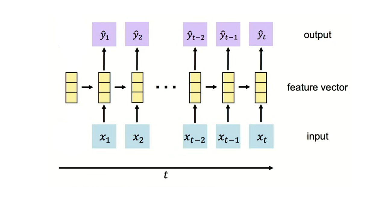
- Sequential processing: An RNN language model processes an input sequence, one element at a time while maintaining an internal state that captures information about previous elements in the sequence. Hence, RNN language models implement sequential processing while standard feed forward neural language models process context words in an input sequence simultaneously in parallel. An input sequence \(x_1, x_2, ..., x_{t-2}, x_{t-1}, x_t\) is processed at different time steps in the network as shown below:
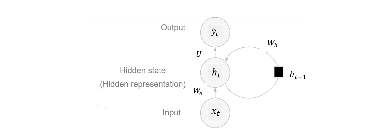
- Recurrent connections: The key feature of RNNs is their recurrent connections. That means, at each time step, an RNN receives an input, updates its hidden state based on both the current input and the previous hidden state, and produces an output. The hidden state serves as a kind of memory that retains information about previous elements of the sequence, enabling the network to capture temporal dependencies and context. The hidden state of an RNN includes a recurrent connection as part of it’s input as shown in the simple RNN below.
Unlike feed-forward neural language models where the predictions are conditioned on a fixed number of words in a sliding context window, recurrent neural network language models condition the predictions on all previous words in the sequence.
Varying sequence length: Since RNNs process one element of an input sequence at a time, RNN language models can handle input sequence examples of varying length compared to feed-forward neural language models, where each input sequence example is made up of a fixed number of words in a context window. RNNs can also produce output sequences of variable length by generating one element of the output sequence at each time step until a termination condition is met.
Parameter Sharing: RNNs share the same set of parameters (weights) across all time steps. This allows the network model size to be the same even when the input sequence gets longer compared to feed-forward neural network models which increase in size when a longer context window is used. Hence RNNs are less complex and generalize well to unseen sequence of text.
RNN Language Model Architechture
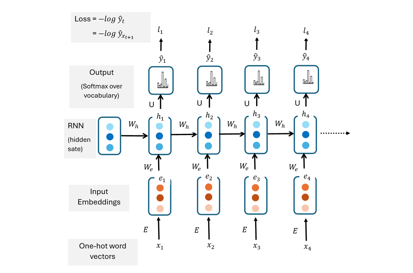
A simple RNN language model architecture consists of an embedding input layer, a hidden state and a softmax output layer. The embedding input layer consists of embeddings that are pre-trained, trained from scratch in the recurrent neural network or fine-tuned.
Training an RNN Language Model
An RNN language model is trained through self-supervised learning where the input data does not need to be explicitly labelled. At any time step, the model uses the next word as the target word to be predicted.
Given a corpus consisting of a sequence of T input words, \(x_1, x_2, x_3, ..., x_{t-1}, x_{t}, x_{t+1}, ... x_T\) represented as one-hot word vectors; an RNN language model can be trained with the sequence of input words. Each input word in the sequence corresponds to a time step.
Forward Pass
Once the input sequence is fed into the RNN language model, the embedding, hidden, and output layers perform computations at each time step t for the forward pass of the training. The ultimate goal of the forward pass is to compute the probability distribution of all the vocabulary words in the sequence.
Embedding layer: A one hot vector representing the word at that time step is transformed by the embedding matrix \(E\) through matrix multiplication into a word embedding, \(e\): \[ e_t = E \cdot x_t \] Hidden state: The hidden state captures information about the current and previous words in the sequence. The current hidden state \(h_t\) is computed using the current input word embedding \(e_t\) and the previous hidden state, \(h_{t-1}\) where the word embedding and previous hidden state are weighted by the matrices \(W_e\) and \(W_h\) respectively:
\[ h_t = g(W_e \cdot e_t + W_h \cdot h_{t-1}) \] where:
- \(W_e\) is the input-to-hidden matrix
- \(W_h\) is hidden-to-hidden matrix
- \(g\) is a non-linear activation function such as \(tanh\) \(relu\) in the hidden state.
Output layer: The output layers first multiplies the hidden state vector \(h_t\) by the hidden-to-output weight matrix \(U\) to obtain a vector whose entries are the unnormalized scores of possible vocabulary words. The resulting vector, often denoted \(z\) is passed into the softmax activation function to generate the probability distribution of the vocabulary words.
\[
\hat{y}_t = softmax(U \cdot h_t)
\] Depending on the RNN task, an output could be predicted at each time step (such as in sequence generation task) or only at the final time step \(T\) (such as in a classification task).
Loss Computation
The output sequence \(\hat{y}\) generated by an RNN can be compared with the actual target sequence \(y\) using cross-entropy or the softmax loss function. The training objective at each time step is to maximize the probability of the correct next word \(w_{t+1}\) given previous words \(w_{1:t}\).
\[ l_t(\theta)= P_{max}(w_{t+1}|w_{1:t})\]
Hence, the training objective at each step is to maximize the softmax probability, \(P(w_{t+1}|w_{1:t})\) or minimize the negative log likelihood of the softmax function. \[\begin{align} l_t(\theta) &= - \sum_{i=1}^V y_{t,i} \log \hat{y}_{t,i} \\ &= - \log \hat{y}_{t,c} \\ &=- \log \hat{y}_{w_{t+1}} \end{align}\]
where:
\(y_{t,i}\) is the \(i\)-th element of the one-hot vector \(y_t = x_{t+1}\) representing the true next word at time step \(t\). \(y_{t,i}\) is 1 for the correct next word and 0 for all other vocabulary words.
\(\hat{y}_{t,i}\) is the probability of the \(i\)th vocabulary word at time step \(t\).
\(\hat{y}_{t,c}\) is the probability of the true next word at time step \(t\).
The loss of the entire training corpus is the average of the losses across the sequence of T words in the training corpus.
\[\begin{align} L(\theta) &= \sum_{t=1}^T l_t(\theta) \\ &= - \sum_{t=1}^T \log \hat{y}_{t,c} \end{align}\]
Backpropagation through Time
Remember that forward pass in a simple RNNs at any time step involves:
- \(h_t = g(W_e \cdot e_t + W_h \cdot h_{t-1})\)
- \(\hat{y_t} = softmax(Uh_t)\)
The loss is the average of the losses at different step:
\[L(\theta) = \sum_{t=1}^T l_t(\theta)\] To find the gradient of the loss with respect to a specific weight, we sum the gradients with respect to that weight from different paths.
- Compute gradient with respect to the weights in the output layer
\[\begin{align} \frac{\partial L(\theta)}{\partial U} &= \sum_{t=1}^T \frac{\partial l_t(\theta)}{\partial U} \\ &= \sum_{t=1}^T \frac{\partial l_t(\theta)}{\partial \hat{y_t}} \cdot \frac{\partial \hat{y_t}}{\partial U} \end{align}\]
- Compute gradient with respect to \(W_h\)
\[ \frac{\partial L(\theta)}{\partial W_h} = \sum_{t=1}^T \frac{\partial l_t(\theta)}{\partial W_h} \\ \] At each time step:
\[\begin{align} \frac{\partial l_t(\theta)}{\partial W_h} &= \frac{\partial t_t(\theta)}{\partial \hat{y_t}} \cdot \frac{\partial \hat{y_t}}{\partial h_t} \cdot \frac{\partial h_t}{\partial W_h} \end{align}\]
But the last part \(\frac{\partial h_t}{\partial W_h}\) can be further expanded because \(h_t\) depends on the previous hidden layer \(h_{t-1}\). Furthermore, \(h_{t-1}\) depends on its own previous hidden layer \(h_{t-2}\), etc and all the hidden layers depend on the same \(W\).
Hence,
\[ \frac{\partial h_t}{\partial W_h} = \frac{\partial h_t}{\partial W_h} + \frac{\partial h_t}{\partial h_{t-1}} \cdot \frac{\partial h_{t-1}}{\partial W_h} \] Similarly, we can further simplify \(\frac{\partial h_{t-1}}{\partial W_h}\) as:
\[ \frac{\partial h_{t-1}}{\partial W_h} = \frac{\partial h_{t-1}}{\partial W_h} + \frac{\partial h_{t-1}}{\partial h_{t-2}} \cdot \frac{\partial h_{t-2}}{\partial W_h} \]
We continue to simplify the derivatives until we find:
\[ \frac{\partial h_1}{\partial W_h} = \frac{\partial h_1}{\partial W_h} + \frac{\partial h_1}{\partial h_0} \cdot \frac{\partial h_0}{\partial W_h} \] When we bring these derivatives \(\frac{\partial h_1}{\partial W_h}\), \(\frac{\partial h_1}{\partial W_h}\), …, \(\frac{\partial h_t}{\partial W_h}\) together, \(\frac{\partial h_t}{\partial W_h}\) and further simplify, we can obtain:
\[ \frac{\partial h_t}{\partial W_h} = \sum_{k=1}^t \frac{\partial h_t}{\partial h_k} \cdot \frac{\partial h_k}{\partial W_h} \]
Hence,
\[\begin{align} \frac{\partial l_t(\theta)}{\partial W_h} &= \frac{\partial t_t(\theta)}{\partial \hat{y_t}} \cdot \frac{\partial \hat{y_t}}{\partial h_t} \cdot \sum_{k=1}^t \frac{\partial h_t}{\partial h_k} \cdot \frac{\partial h_k}{\partial W_h} \\ \end{align}\]
where:
\[ \frac{\partial h_t}{\partial h_k} = \prod_{i=k+1}^T \frac{\partial h_i}{\partial h_{i-1}} \]
- Compute gradient with respect to \(W_e\)
The gradient of the loss with respect to the weight matrix \(W_e\) used for weighting the input embeddings can be derived in the same way we derived the gradient with respect to \(W_h\).
Parameter Update
The stochastic gradient descent rule is used to update the weights of the RNN language model as follows:
\[ \theta ← \theta - α ⋅ \frac{\partial L(θ)}{\partial \theta} \]
Challenges of RNNs
Training Efficiency: RNNs are computationally slow especially when a large corpus is used to train the model. The computation is slow because of the sequential nature of RNNs where a single input in a sequence is fed into the model at each time step, with no parallelization. Additionally, there are several computations in each time step.
Difficulty with Learning Contextual Information:: It is generally difficult for RNNs to learn contextual information far in the sequence partly due to the vanishing gradient or exploding grading problem. A vanishing gradient problem is when the gradient with respect to weights in earlier time steps diminishes due to derivatives in the chain rule being less than 1. Small gradients at earlier steps means the weights are almost optimal. This implies the network is not learning much for the earlier inputs, hence long-term contextual information in the sequence is not learned or captured by the network.
Understanding Backpropagation and Gradient Instability Issues
To understand the gradient instability issues such as the vanishing gradient and gradient explosion problems, it is vital to understand how backpropagation works in computing gradients with respect to weights in each layer of a neural network.
Let’s consider a simple feed-forward neural network with an input layer, a hidden layer and an output layer where:
- \(x\): Input to the neural network
- \(W_1\): Weight matrix for the first layer
- \(W_2\): Weight matrix for the second layer
- \(h = g(W_1 x)\): Output of the hidden layer after applying activation function \(g\)
- \(z = W_2 h\): Input to the activation function \(g\)
- \(\hat{y} = g(z)\): Output of the neural network after activation
- \(L(\theta)=L(\hat{y}, y_{true})\): Loss function comparing predicted output \(\hat{y}\) with true labels \(y_{true}\)
The two-layer neural network diagram looks like this:
\(x \rightarrow W1 \rightarrow z_1 = W_1x \rightarrow h = g(z_1) \rightarrow W_2 \rightarrow z_2 = W_2 h \rightarrow \hat{y} = g(z_2) \rightarrow L\)
Our goal is to compute the gradient or derivative of the loss function with respect to the weights (\(W_1\) and \(W_2\)) in the hidden and output layers respectively.
We need to trace the input and outputs in the hidden and output layers and use that relationships between the inputs and outputs to compute the gradient in each layer. These relationships can be captured as a composite function which can then be differentiated using the chain rule.
Gradient of the loss function with respect to weights in the output layer: We want to compute the derivative of the loss with respect to \(W_2\).
- \(W_2\) is input to \(z_2\); \(z_2\) is input to \(\hat{y} = g(z_2)\) and \(\hat{y}\) is input to \(L\).
- With backward differential using the chain rule:
\[ \frac{\partial L(\theta)}{\partial W_2} = \frac{\partial L(\theta)}{\partial \hat{y}} \cdot \frac{\partial \hat{y}}{\partial z_2} \cdot \frac{\partial z_1}{\partial W_2} \]
Gradient of the loss function with respect to weights in the hidden layer: Similarly to the process of computing gradient with respect to the weights in the output layer, we need to trace the inputs and outputs from that layer to the loss function. Remember that \(W_1\) is a weight matrix containing the weights for the hidden layer.
\[ \frac{\partial L(\theta)}{\partial W_1} = \frac{\partial L(\theta)}{\partial \hat{y}} \cdot \frac{\partial \hat{y}}{\partial z_2} \cdot \frac{\partial z_2}{\partial h} \cdot \frac{\partial h}{\partial z_2} \cdot \frac{\partial z_1}{\partial W_1} \] The vanishing gradient problem: For a deep neural network, the gradient may diminish exponentially as we move backward and compute gradients with respect to earlier weights especially if some of derivatives in the chain rule are less than 1. The derivatives of activation functions such as sigmoid are in the range of 0 and 1.
Earlier gradients require more derivatives to be multiplied in the chain rule and when we multiply more small numbers between 0 and 1, the results become smaller and smaller, hence the gradient with respect to earlier weights vanishes as the network gets deeper. The vanishing of gradients with respect to earlier weights in a deep neural networks is called the vanishing gradient problem. As a results, the earlier parameters update slowly and much learning does not happen for the earlier layers.
The gradient explosion problem: This is the opposite of the vanishing gradient problem, where the gradient grows uncontrollably as the gradients propagate backward through many layers in the deep neural network. This happens mostly when the derivatives of the activation functions in the chain rule are greater than 1, depending on the choices of the activation functions.
Solution to Exploding and Vanishing Gradient
Activation functions such as sigmoid and tanh in deep neural networks can result to vanishing gradient while leaky Relu can result to exploding gradient. The following approaches can be used to mitigate exploding and vanishing gradient problems.
Gradient clipping: This involves setting threshold values and rescaling the gradients if they exceed this threshold.
Weight initialization: Xavier/Glorot initialization is used to set the initial weights such that the variance of the gradients remains consistent across layers, helping to prevent vanishing gradient in deep networks. Random initialization of weights with parameters drawn from a normal distribution with a mean of zero and small variance (for example: \(\mu =0; \sigma = 0.1\)) ensures the weights are small and not too large, which can lead to gradient instability or explosion during training.
Variants of RNNs: Advanced architectures like Long Short-Term Memory (LSTM) and Gated Recurrent Unit (GRU) have been developed to mitigate the vanishing gradient problem in RNNs, by introducing gating mechanisms that allow the network to selectively retain or update information in the hidden state, thus enabling better learning of long-range dependencies.
RNNs for Part of Speech (POS) Tagging
The RNN architecture for POS is as follows:
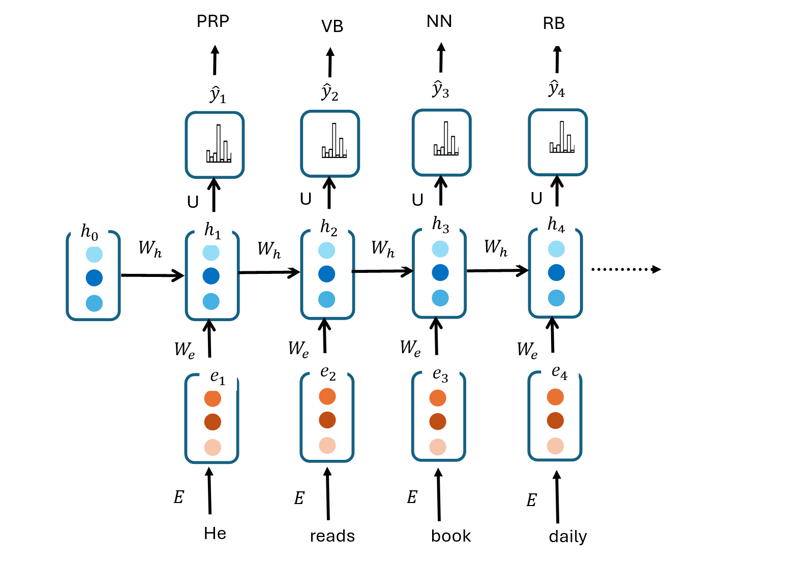
The RNN model is trained with a sequence of text where each word in the corpus is labeled with it’s corresponding POS. For example, the sequence of words He reads books daily. could be tagged as follows:
- “He” - PRP (pronoun, personal)
- “reads” - VBZ (verb, 3rd person singular present)
- “books” - NNS (noun, plural)
- “daily” - RB (adverb)
During model training, word embeddings \(e_1, e_2, ..., e_T\) corresponding to a sequence of words \(w_1, w_2, ..., w_T\) are fed sequentially into the RNN. At each time step, the current hidden state \(h_t\) is updated with both the current input embedding \(e_t\) and the previous hidden state \(h_{t-1\).
The softmax output layer then applies weights to the output of the hidden layer to obtain a vector of pre-activation scores that are further processed by the softmax activation function to generate the probability distribution of part-of-speech tags.
To maximize the probability of the actual POS tag label or to minimize the difference between the actual and predicted POS tag, the probability of the actual label is then used to compute the softmax loss or cross entropy loss: \(l_t = - \log P(POS_{true}|x_1, x_x, ..., x_t)\). The gradient of the softmax loss with respect to each weights in the network is computed using backpropagation through time. The stochastic gradient descent optimization is used with the gradients update the weights in the network.
RNNs for Sequence Classification
RNNs can be used for classification of each entire sequence example instead of the words in the sequence. The architecture for RNNs for sequence classification is as follows:
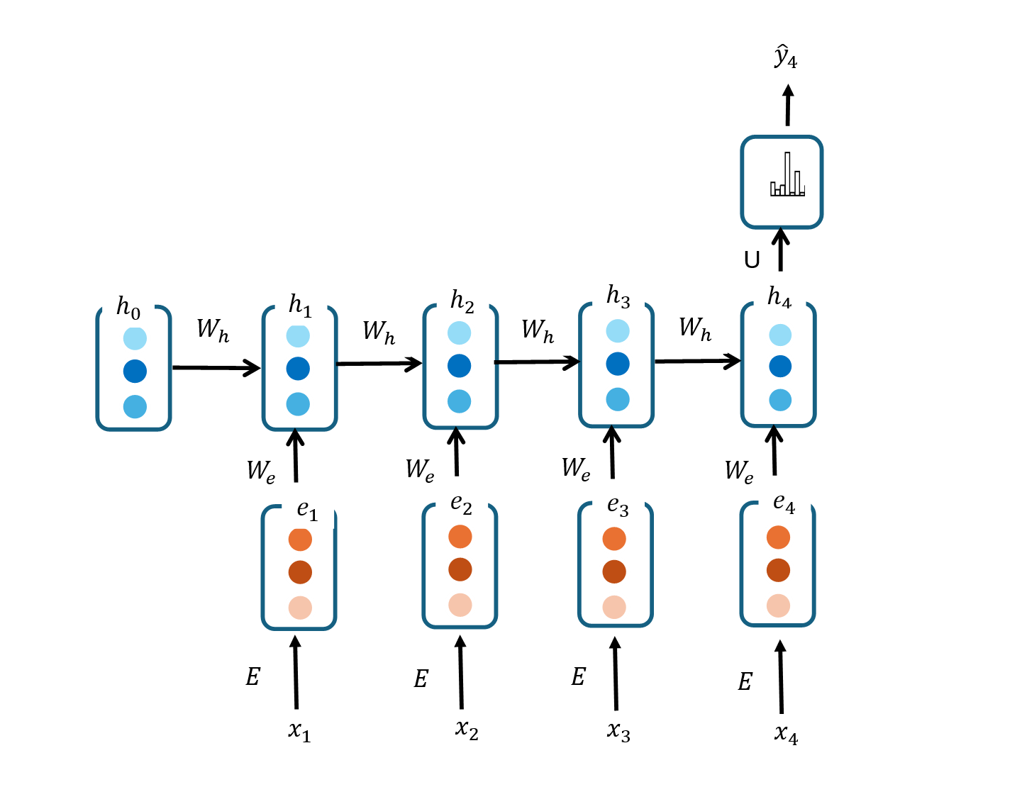
Word embeddings of words in the input sequence are sequentially passed as input into the RNN. At each time step, the current hidden layer takes the current input and the previous hidden state as input. For a sequence classification use case such as sentiment analysis of documents, only the last hidden layer is used as input into the output layer.
The output layer generates probability distribution of sentiments (positive, neutral, negative) if the output layer as a softmax activation function. The probability of the correct sentiment (positive or negative) is generated if the output layer has a sigmoid activation function. Forward propagation is used to generate the probabilities of the sentiments.
The loss function of an RNN for classification maximizes the probability of the correct class. The gradient of the loss function with respect to each weight in the network is computed using backpropagation through time. The gradients are then used with the stochastic gradient descent rule to update the weights in the network to minimize the cross-entropy loss, which captures the difference between the actual and predicted label. The weights updated are the weights in the weight matrices weight matrix \(W_e\), or \(W_h\) and \(U\).
RNNs for Text Generation
RNNs with the following architecture can be used for autoregressive generation.
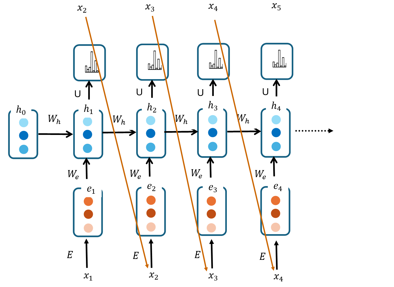
RNN language models are suitable for text generation because their internal state capture contextual information about previous words.
The RNN language model for text generation is trained normally with a large corpus by sequentially feeding the network with embeddings of words in the input sequence. At each time step, the RNN predicts the probability distribution over the vocabulary.
The predicted probability of the correct word is used to compute the cross-entropy loss. The gradient of the cross entropy loss with respect to each weight in the model is computed using backpropagation through time. The gradient is then use to update the weights using stochastic gradient descent while minimizing the loss function.
At inference or prediction time, the trained RNN language model is fed with an initial token or prompt to generate a output sequence of text. Two phases are involved in generating text called sequence generation and autoregressive generations.
Sequence generation: During this phase, the embedding of an initial input token is used to generate an output token. Alternatively, embeddings of words in an initial prompt could be sequentially fed into the RNN language model to generate an output sequence. Prompts are a few words tokenized into a sequence of words.
At any time step, when embedding of the an input token is fed into the RNN language model, the hidden layer uses the previous hidden state (contextual information) and the embedding of the current input token to compute the hidden state.
The hidden state is then transformed and used by the output layer to generate a probability distribution over next words (vocabulary words). The word with the highest probability is the generated as the predicted word.
Autoregressive generation: After generating the initial output sequence from the prompt, the last generated token from this output sequence is used as the starting point for autoregressive generation, where each token are sampled from the predicted probability distribution and used as input into the next time step.
The sampling of tokens from the predicted probability distribution could be done using greedy sampling or stochastic sampling.
Greedy sampling: This involves choosing the token with the highest probability at each generation step. Greedy sampling is deterministic.
Stochastic sampling: This involves choosing tokens based on their probabilities, allowing for variability and randomness in token selection. Each time a token is selected at time step \(t\), it becomes an input in the next time step \(t-1\). This process continues until the stop criteria is reached.
Temperature sampling: Note that a temperature parameter could be introduced in the softmax activation function in the output layer to control the randomness and diversity of generated token. The temperature parameter influences the diversity and creativity of generated text.
With temperature sampling, we divide the logit or input vector \(z\) of the softmax activation function in the output layer by the temperature parameter \(\tau\).
Hence, the probability distribution
\[\begin{align} \hat{y} &= P(y_t | \text{context}) \\ &= softmax(\frac{z}{\tau}) \\ \end{align}\]
By modifying \(\tau\) practitioners can control the extend to which the generates novel and coherent sequences.
Temperature Adjustment:
- τ = 1.0 (neutral temperature): The ditribution does not change resulting to a balanced mix of probable tokens based on the softmax distribution.
- τ = 2.0 (high temperature): The model explores a broader range of tokens, including less probable ones, leading to more diverse outputs.
- τ = 0.5 (low temperature): The model generates more deterministic outputs, focusing on tokens with the highest probabilities.
The beautiful thing with RNNs is that the predictions at each time steps are based on the previous hidden state or historic context. Conditioning predictions on preceding words is useful for generating meaningful text.
Bidirectional RNNs
Bidirectional RNNs are neural networks where predictions are conditioned on both past and future context instead of on past context only, as in traditional RNNS. The network processes sequences using both right-to-left and left-to-right propagation as shown in the bidirectional RNNS architecture below:
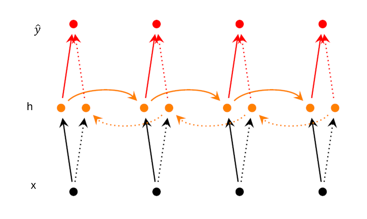
So, at each time step, both past and future context is used for predictions. The network has two hidden states at each time step capturing both past and future context. Therefore, the networks provides a better understanding of the sequence compared to traditional RNNs. This explains why a bidirectional RNN is better for tasks such as sentiment analysis where the understanding of the entire sequence is necessary.
At time step t, the hidden states for the forward and backward RNN are combined in some way such as through concatenation, element-wise averaging or max. The resulting final hidden state is processed by the output layer. For a classification use case, the softmax or sigmoid activation in the output layer is used for generating predictions conditioned on past and future context.
Long Short-Term Memory (LSTM)
Why LSTM?
RNNs suffer from the vanishing gradient problem, which makes it difficult for RNNs to capture long-term dependencies in sequential data. The vanishing gradient problem can be addressed in various ways including the use of Relu activation functions in the hidden layers instead of sigmoid which prevents the gradient from shrinking if the input into the Relu function is greater than 0. Initializing parameters using random values drawn from a normal distribution with a mean of zero and small variance close to zero (e.g. 0.1) also prevents the gradients from shrinking.
What is an LSTM?
An LSTM is a robust and complex architecture for addressing the vanishing gradient problems that limits RNNs from learning long-term dependencies. LSTM is an extension of the RNN architecture designed to capture relevant long-term context by enabling the network to learn only contextual information that is needed and forget information no longer needed.
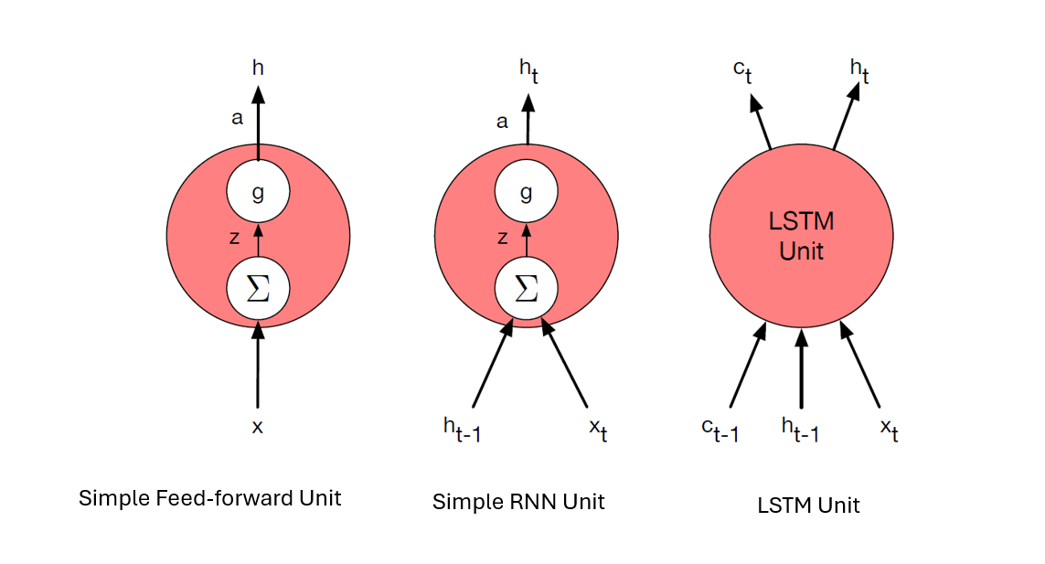
LSTM vs FFNN and RNN Units
Compared to a FFNN or an RNN, an LSTM unit has context layer explicitly specified in the architecture in addition to the recurrent hidden layer. The LSTM network also has gates that control the flow of information into and out of the computation unit of the network. The gates are implemented through additional weights that transform the input, previous hidden layer and context layer into the current hidden state.
LSTM unit as a Computation Graph
At each time step t, an LSTM unit is fed with the input \(x_t\), the hidden state \(h_{t-1}\), and the previous context (cell state) \(c_{t-1}\). Within the LSTM unit, gates or gated cells are used to transform \(x_t\), \(h_{t-1}\), and \(c_{t-1}\) to obtain an updated cell state \(c_t\) and hidden state \(h_t\) as shown in the computation graph below.
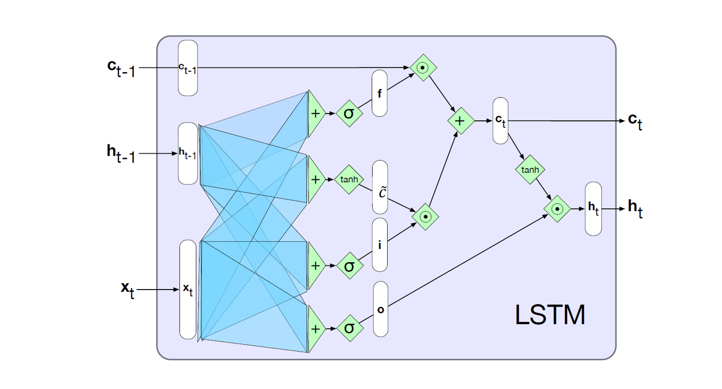
Gates in an LSTM Unit
Gates are basically functions that transform information inside the LSTM unit. Each gate is a feed-forward layer with a sigmoid activation followed by an element-wise multiplication with the information being gated (or filtered). There are three gates inside the LSTM unit:
- The Forget Gate (\(f_t\)): The forget gate determines what information from \(c_{t-1}\) should be retained or discarded. The forget gate transforms and combines the input \(x_t\) and previous hidden state \(h_{t-1}\), then, passes the result into a sigmoid activation function to generate a vector whose entries are between 1 and 0.
\[ f_t = \sigma(W^{(f)} x_t + U^{(f)}h_{t-1}) \]
- The Input Gate (\(i_t\)): The input gate regulates how much of the new information \(\tilde{c}_t\) should be added to the information retained from \(c_{t-1}\) to obtain an updated cell state \(c_t\).
\[ i_t = \sigma(W^{(i)} x_t + U^{(i)}h_{t-1}) \]
New information \(\tilde{c}_t\) at time step t is the normal information computed for a traditional RNN:
\[ \tilde{c}_t = \tanh(W^{(c)} x_t + U^{(c)}h_{t-1}) \] \(\tilde{c}_t\) is also called memory cell.
- The Output Gate: The output gate determine how much information in the updated cell state \(c_t\) is relevant output at time step t or should be exposed as the hidden state \(h_t\).
\[ o_t = \sigma(W^{(o)} x_t + U^{(o)}h_{t-1}) \]