Probability is a branch of mathematics that studies randomness and uncertainty. As a concept, probability measures uncertainty associated with an outcome. It is the numerical value that measures the chance or likelihood that an event will occur. Probability provides the connection between observed data in the past and unknown outcomes in the future. Probability helps us understand how likely an event will occur.
For instance, given the sales data for the past three years, how likely will next month’s sales be greater than last year’s average sales? Our understanding of probability is useful for answering questions such as, what are the odds that a particular team will win an upcoming soccer game?
The Applications of Probability?
Probability is the foundation of theoretical probability distributions and probabilistic modeling. Probability concepts are used in constructing theoretical distributions, to understand the chances associated with various outcomes. In probability modeling, the principles of probability enable us to find the uncertainty associated with possible model parameters.
Probability is the foundation of statistical inference. Probability helps us answer questions involving statistical inference such as, to what extent can we say that a sample with an observed sample statistic came from a defined population with known parameters? How likely are two observed data samples from the same population? In other words, is there a statistical significant difference between two populations? To be more concrete, statistics could be used to answer questions such as, is there a statistical significant difference between the salaries of male and female data scientist?
In this era, probabilistic and statistical methods are widely applied in almost all fields of life, making it imperative for workers, managers, scientists, engineers, or anyone to acquire some basic knowledge of probability theory. The knowledge of probability concepts helps us to quantify the uncertainties, chances or likelihoods associated with various outcomes in situations where one out of a finite number of possible outcomes may occur.
Statistical Experiments
The word “experiment” in statistics does not refer to a scientific experiment in a laboratory. A statistical or random experiment is any activity or process whose outcome is uncertain. A statistical experiment is also called a trial. The result of a random experiment is called an outcome. An experiment is a process that generates well-defined outcomes.
Examples of random experiments include:
randomly selecting students in a class and observing their grades,
tossing a coin,
rolling a dice,
testing whether a product is good or defective,
observing whether those who click an ad would buy a product or not,
and so on.
Events and Sample Space
An event is a collection of the outcomes of a random experiment. That is, an event consists of one or more outcomes of an experiment. A sample space is a set of all distinct possible outcomes of a random experiment. A sample space is denoted by S. A sample space can be listed or enumerated if the outcomes are discrete. For example, if we are interested in describing whether a business website visitor would buy or not buy, our sample space would be: \[S = \text{\{Buy, Not Buy}\}\] In another situation where we are testing for good or bad products, the sample space would be: \[S = \text{\{Good, Bad}\}\]
Suppose gas station A has two gas pumps and station B has two as well. If the events in the sample space consist of the number of gas pumps in use at station A and station B at any time, then the events in the sample space can be listed as follows: \[S = \text{\{(0, 0), (0, 1), (0, 2), (1, 0), (1, 1), (1, 2), (2, 0), (2, 1), (2, 2)}\}\]
On the other hand, listing all possible outcomes in a sample space is impossible when the outcomes are continuous. In such a situation, a rule can be used to specify the sample space. For example, if we want to randomly select students and describe their scores in a data science course, the sample space could be written as follows (X represents the score of a randomly selected students): \[S = \text{\{0 =< X >=100}\}\]
An event is a subset of a sample space and consists of an outcome or a collection of outcomes. A simple event consists of one outcome, while a compound event consists of two or more outcomes. In the situation where the number of pumps from station A and station B is observed, the sample space is: \[S = \text{\{(0, 0), (0, 1), (0, 2), (1, 0), (1, 1), (1, 2), (2, 0), (2, 1), (2, 2)}\}\]
There are 9 simple events in this sample space. For example, one of the simple events, E1 = {(0, 0)}. An example of a compound event could be an event, A, describing outcomes where the total number of pumps in use for both stations is 2: \[A = \text{\{(0, 2), (1, 1), (2, 0)}\}\] Another compound event B could be that the number of pumps in use is the same for both stations:
\[B = \text{\{(0, 0), (1, 1), (2, 2)}\}\]
The probability of each event in a sample space could be calculated or assigned. For example, the probability that the number of pumps used in station A is equal to the number of pumps used in station B is 3/9 or 0.33. The subsequent sections provide more guidance on how to calculate the probability of an event.
Types of Probability
Different approaches are used to assign or compute probability, resulting in different types of probability. Various approaches for assigning probability include:
the classical approach
empirical approach
subjective approach
Classical Probability
The classical approach assigns probability based on prior knowledge of possible outcomes in the sample space. It assigns probability a priori without necessarily observing an event or the outcome of a random trial because the nature of the experiment or process allows us to envision all the possible outcomes in the sample space. For example, the probability of getting a head when a fair coin is tossed is known a priori. The classical approach assumes that all outcomes in the sample space are equally likely to occur.
Definition of Classical Probability
Classical probability is the number of favorable or desired outcomes divided by the total number of possible outcomes in the sample space. That is, according to the classical approach: \[\text{Probability}=\frac{\text{Number of Favorable Outcomes}}{\text{Total number of possible Outcomes}}\]\[P(E)=\frac{n(E)}{n(S)}\] This formula implies that, for an event E in a sample space S, the probability of the event P(E) can be computed using the classical approach by counting the number of outcomes in the event, n(E), and dividing that by the total number of possible outcomes, n(S).
Given a sample space, \(S = \text{\{1, 2, 3, 4, 5, 6,7, 8, 9, 10}\}\), where the outcomes in the sample space equally likely, if an event E is defined as outcomes that are greater than 5 in the sample space, then, the probability of the event is calculated as: \[P(E)=\frac{\text{Number of outcomes greater than 5}}{\text{Total number of possible outcomes}}\]\[P(E)=\frac{4}{10}=0.4\]
Use Cases for the Classical Probability Approach
The following are examples of situations where the classical approach can be used to assign probabilities:
If a fair coin is tossed once, the probability of getting a head is 1/2 or 0.5.
If a fair dice is rolled once, the probability of rolling a 2 is 1/6.
If there are five male students in a class of 15 students, if all students have an equal chance of being selected, then the probability of randomly selecting a male student is 5/15 or 0.33.
The Assumptions of the Classical Probability Approach
The classical approach to probability was developed and applied historically around the 17th century to games of chance such as cards and dice. The classical or chance models can describe mutually exclusive, collectively exhaustive, and equally likely outcomes (Wentzel, 1982).
Assumption #1
The events in the experiment must be mutually exclusive. That means the events in an experiment do not overlap. Given the sample space, \(S = \text{\{1, 2, 3, 4, 5, 6,7, 8, 9, 10}\}\). The following event; \(E1 = \text{\{1 =< X <= 5}\}\) and \(E12= \text{\{5 < X <= 10}\}\) in an experiment are mutually exclusive because they do not overlap. The outcomes of an experiment are also said to be mutually exclusive only if one outcome can occur at a time.
For example, suppose a shop allows customers to make payments only through credit card, debit card or cash, and we are interested in computing the probability of that a customer with use a specific payment method for a transaction. These payment methods are mutually exclusive only if one method of payment could be used per transaction. If two or more methods of payments are allowed to be used per transaction, then these payment methods are mutually exclusive. If the methods of payment are equally likely, then we can use classical probability to compute the probability of making a payment through a specific payment method.
Assumption #2
The events in the experiment must be collectively exhaustive. Events in an experiment are collectively exhaustive if the events cover the entire sample space. Given the sample space, \(S = \text{\{1, 2, 3, 4, 5, 6,7, 8, 9, 10}\}\); the events \(E1 = \text{\{1 =< X <= 5}\}\) and \(E12= \text{\{5 < X <= 10}\}\) are collectively exhaustive because the events cover the entire sample space. If events are collectively exhaustive and mutually exclusing, then the sum of their probabilities must be 1.
Assumption #3
The classical approach can be applied only to situations where the probabilities of outcomes can be determined a priori. If we lack prior knowledge of all possible outcomes in the sample space, then it is not possible to use the classical approach to compute the probabilities of events in the sample space.
Assumption #4
The outcomes of the experiment must be equally likely. The classical approach is not suitable for scenarios with outcomes that are not equally likely. When outcomes are not equally likely, it means some outcomes are more likely to occur than others, such as when a biased or unfair coin is tossed.
Suppose we want to find the probability that a United Airlines flight from Denver to Durango would arrive late. The event in this situation is late arrival, \(E={\{late}\}\) and the sample space is \(S = \text{\{late, not late}\}\). If we use the classical approach, the probability of late arrival will be, \[P(E)=\frac{n(E)}{n(S)}=\frac{1}{2}=0.5\]
However, in real life, given the sample space \(S = \text{\{late, not late}\}\) representing the outcomes of a United Airlines flight, the outcomes are not usually equally likely. Hence it would not be suitable to use the classical approach to estimate the probability of a late flight. That means, we cannot use the classical approach to say that the probability of flight arriving late is 0.5. We could instead use observed data and the relative frequency or proportion of late flights to estimate the probability that a flight would arrive late. This approach where observed data is used to compute the probability of an event is called empirical probability.
Empirical probability
The empirical approach assigns probability using observed or empirical data, usually collected through repeated trials. In real life, empirical data is collected through surveys, observations, or experimental studies. The empirical approach is also called the frequentist approach, which defines probability as relative frequency in the long run. The empirical approach defines probability of an event as the limit of the number of times the event occurs divided by the total number of trials, as the number of trials becomes very large. In simple terms: \[P(E)=\frac{\text{Number of times an event occurs}}{\text{Total number of trials}}\] The empirical approach considers the probability of an event to be the relative frequency of the event after several repeated trials of a random experiment. According to the empirical approach, you can estimate the probability of an event occurring using the proportion of times the event occurred in the past.
The empirical perspective of probability is based on the law of large numbers, which states that as the number of trials increases, the empirical probability of an outcome approaches its theoretical limit or actual probability. In other words, as the number of trials in a random experiment increases, the average of the outcomes will approach the expected value. That means, in the long run, the relative frequency of each outcome stabilizes.
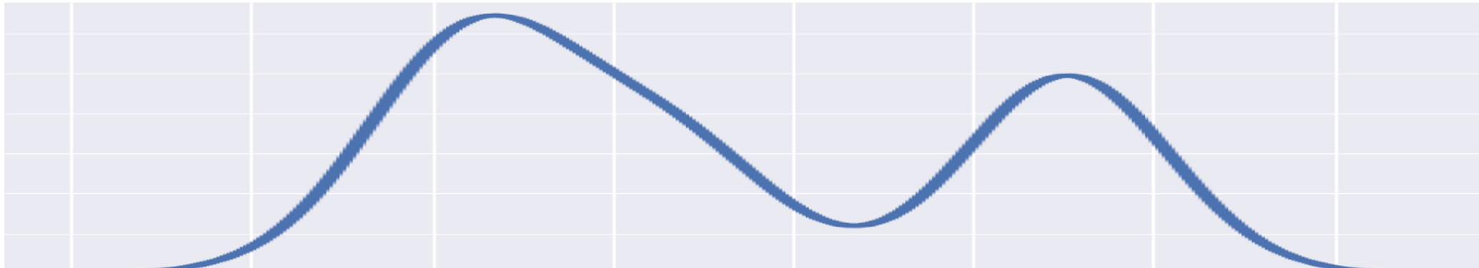
Below is a simulation in Python that illustrates the empirical approach and the law of large numbers when a coin is tossed. The sample space \(S = \text{\{0, 1}\}\) represents the possible outcomes of the coin tossing experiment where 0=tail and 1=head. For each run, we will randomly draw a value from the sample space n times. We will implement several runs where each run has a different number of trials: \(n\_list = \text{\{5, 50, 100, 500, 1000, 10000}\}\)
We will then analyze how the probability of obtaining 1=head changes as the number of trials increases across the runs. Each record or row in the table below represent information (number of trials and probability of obtaining a head) for a specific run.
Code
import pandas as pd import numpy as npsample_space = [0,1]n_list = [5, 50, 100, 500, 1000, 10000]probability_head_list = []np.random.seed(3)for n in n_list:# randomly draw n values trials = np.random.choice(sample_space, size=n)# compute the probability of obtaining a head prob_head = np.mean(trials) probability_head_list.append(prob_head)# zip the data and create a dataframe data =list(zip(n_list, probability_head_list))data = pd.DataFrame(data, columns=["number_of_trials", "probability_head"])data.style.set_table_styles([dict(selector='th', props='min-width: 60px;'),]).format(precision=2)
number_of_trials
probability_head
0
5
0.40
1
50
0.48
2
100
0.45
3
500
0.46
4
1000
0.48
5
10000
0.50
As the number of trials increases, the probability of obtaining a head converges or gets closer to 0.50.
Therefore, the probability of tossing a fair coin and obtaining a head is 0.5. That means if a fair coin is tossed several times, the head will show up 50% of the time. This is how the empirical approach interprets probability.
The empirical approach considers probability to be objective since the assignment of probabilities is based on counts of observed outcomes of a random experiment. This approach is great for certain types of problems where the collection of data from a random or statistical experiment is feasible. For example, observed data can be used to find the probability that a flight from Denver to Durango will arrive late as follows: \[P(E)=\frac{\text{Number of times a flight arrived lates}}{\text{Total number of flights}}\]
There are certain types of problems that are not suitable for the empirical probability approach. For example, If you wanted to know the probability that a Republican candidate for the presidential election will win the election, you won’t not have enough trials to satisfy the definition of empirical probability. The empirical approach is applicable only when the outcome of an experiment can be observed repeatedly.
Empirical probability is considered objective as it depends on the counts of an observed event after several trials. When it is not possible to use objective probability to measure uncertainty, subjective probability could be used.
Subjective Probability
Subjective probability can be used to assign the probability that a Republican candidate for the presidential election will win an upcoming election. Subjective probability depends on the degree of belief of an individual about the outcomes of an experiment.
The subjective approach to probability assigns probability based on an individual’s informed judgment about the chances or likelihood that an event will occur.
For example, a development team of a new product may assign a probability of 0.7 that the product will be successful, while a more pessimistic manager assigns 0.2 as the probability that the product will be successful. Subjective probability varies from individual to individual and depends on experience, personal opinion, and the analysis of circumstances that could impact the outcome of interest.
Subjective probabilities are used as prior probabilities in Bayesian modeling. The subjective approach can be helpful when there is insufficient past data or when it is not feasible to generate sufficient data at the time when the probability of an outcome needs to be assigned. Subjective probabilities are helpful when the classical and empirical approaches are not possible.
The Rules of Probability
Set theory can be applied to events because an event is a set of outcomes. So, the complements, unions and intersections of events can be computed. The probability of an event A is written as P(A).
The Complement Rule
The complement of event A is an event \(A^c\), consisting of all the outcomes in the sample space S that are not in event A. An event and its compliment are mutually exclusive and collectively exhaustive, hence, the sum of the probability of an event and the probability of its compliment must be 1. That is, \(P(A) + P(A^c) = 1\), therefore, \[P(A^c) = 1 – P(A)\]
Events and their complements are commonly used to calculate odd ratios:
The odds in favor of an event A is defined as: \[\frac{P(A)}{P(A^c)} = \frac{P(A)}{1 – P(A)}\]
The odds against an event A is defined as: \[\frac{P(A^c)}{P(A)} = \frac{1 – P(A)}{P(A)}\]
The General Addition Rule
The addition rule involves the union of events. The union of events A and B is denoted as \(A \cup B\), which is the same as \(\text{A or B}\). The union of two events consists of all outcomes that are either in A or B or both. According to the general addition rule, the probability of the union of two events is written as: \[P(A \cup B) = P(A) + P(B) - P(A \cap B)\]\(A \cap B\) stands for the intersection of two events, A and B, and consists of all the outcomes that are common in both events A and B. The probability of the intersection of two events, P(A ∩ B) is also called joined probability, defined as the probability of events A and B occurring together. More details about joined probability will be provided under the multiplication rule.
The Special Addition Rule
In a special case where events are mutually exclusive, \(P(A \cap B) = 0\) because mutually exclusive events are disjointed or cannot co-occur. That is, the intersection of mutually exclusive events is an empty set. \(A ∩ B = ϕ\). Since mutually exclusive events have no intersection or do not overlap, the addition rule for mutually exclusive events is written as: \[P(A \cup B) = P(A) + P(B)\]
Events \(A1, A2, A3, …,An\) are considered collectively exhaustive if they cover all possible outcomes of an experiment. The union of collectively exhaustive events makes up the entire sample space.
The General Multiplication Rule
The general rule of multiplication is also called the product rule. This rule allows us to compute the joined probability of events or the probability of the intersection of events. Note that \(P(A \cup B)\), \(P(A, B)\) or \(P(\text{A and B})\) all stand for joined probability. The joined probability of events A and B is defined as: \[P(A \cap B) = P(A/B)P(B) = P(B/A)P(A)\]
The Special Multiplication Rule
If event A is independent of event B, then \(P(A) = P(A|B)\) and \(P(B) = P(B|A)\). Therefore, the general rule of multiplication is simplified to: \[P(A \cap B) = P(A)P(B)\]
The Chain Rule
The chain rule generally extends the product rule to more than two variables or events. For instance, the joint probability of several events \(A1, A2, A3, …, An\) is written as: \[P(A1, A2, A2, …, An) = P(A1|A2, A3,…,An)P(A2|A3,…,An)…P(An)\] or \[P(A1, A2, A2, …, An) = P(A1)P(A2|A1)P(A3|A2, A1)…P(An|An-1…A1)\] For independent events, \(P(Ai|Aj) = P(Ai)\), hence, the chain rule is simplified to: \[P(A1, A2, A2, …, An) = P(A1)P(A2)P(A3)…P(An)\]
The chain rule is very useful in constructing Bayesian networks.
Conditional Probability
Conditional probability is the probability of an event A, given that another event B has already occurred. The notation for conditional probability is \(P(A|B)\), which means “the probability of A given B.”
Conditional Probability and the Multiplication Rule
Conditional probability is derived from the general rule of multiplication. That is: \[P(A ∩ B) = P(A/B)P(B)\]\[⇒ P(A/B) = P(A \cap B)/P(B)\]
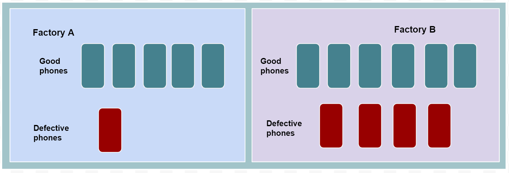
\(P(A/B)\) is the conditional probability of A given B, provided P(B) > 0. To illustrate the idea of conditional probability let’s suppose a company has two factories, A and B, that manufactured a total of 16 phones as shown below.
All the 16 phones manufactured in the past by the two factories were tested. It was found that 5 out of 16 phones produced by the company (two factories) were defective. Furthermore, 1 out of 6 phones produced in Factory A were defective while 4 out of 10 phones produced by Factory B were defective.
We can find the probability that a phone produced by this company will be defective as follows: \[P(\text{Defective Phone})=\frac{\text{Number of defective phones}}{\text{Total number of phones}}\]\[P(\text{Defective Phone})=\frac{5}{16} = 0.31\] If we are interested in finding the probability that a phone is defective given that it was produced by Factory A, then we are in other words trying to find the conditional probability of a phone being defective given factory A, \(P(\text{Defective Phone|Factory A})\).
Conditional probability simply involves computing probability of an event within a subpopulation. So,the conditional probability of a phone being defective given that the phone is produced by Factory A can be calculated as follows:
\[P(\text{Defective Phone|Factory A})=\frac{\text{Number of defective phones in Factory A}}{\text{Total number of phones in Factory A}}=\frac{1}{6}=0.17\] We can also find the conditional probability that a phone is defective given that it is produced by Factory A, using the conditional probability formula derived from the multiplication rule as follows:
\(P(\text{Defective Phone} \cap \text{Factory A})\) is the probability that a phone is defective and is produced by Factory A. This probability is calculated as:
\[P(\text{Defective Phone} \cap \text{Factory A}) = \frac{\text{Number of defective phones in Factory A}}{\text{Total number of phones in the entire company}} = \frac{1}{16}\]
\(P(\text{Factory A})\) is the probability that a phone is produced in Factory A. This probability is written as:
\[P(\text{Factory A}) = \frac{\text{Number of phones in Factory A}}{\text{Total number of phones in the entire company}} = \frac{6}{16}\] Therefore, \[P(\text{Defective Phone|Factory A})=\frac{P(\text{Defective Phone} \cap \text{Factory A}}{P(\text{Factory A})}=\frac{1/16}{6/16}=\frac{1}{6}=0.17\] The conditional probability obtained when we use the conditional probability formula derived from the multiplication rule is the same as the conditional probability obtained when calculate the probability of defective phones only within the subpopulation, Factory A. Hence, it is more intuitive to think of conditional probability as probability within a subpopulation. That means, conditional probability of A given B is the probability A within the subpopulation, B.
Estimating Conditional Probability Using a Dataset
A conditional probability problem may not always be framed as a word problem. In some cases, we may be required to estimate conditional probability using a dataset provided. The columns of the dataset are considered to be random variables and the records or row values in the dataset are the outcomes associated to the random variable.
Let’s consider a_i to be one of the unique outcomes associated with the random variable A and b_j to be one of the unique outcomes associated with the random variable B. To find the conditional probability, P(A=a_j|B=b_j), we can select a subset of the data for which the condition B=b_j is true, then find the probability of A, P(A=a_i) in the subdataset. That means P(A=a_i|B=b_j) could be computed as the number of times A=a_i occurs in the subdataset divided by the number of cases in the subdataset.
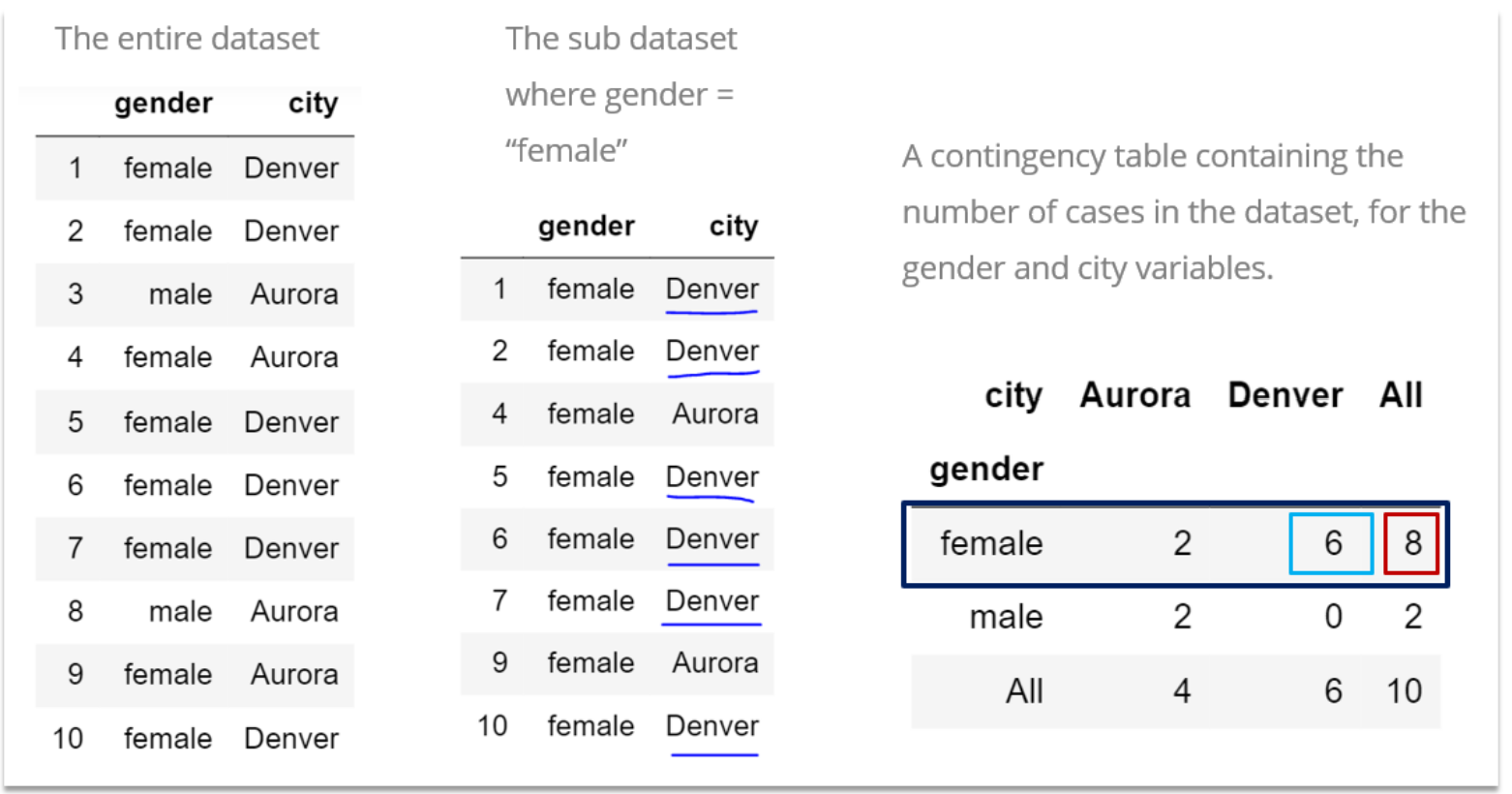
Let’s make the above explanation concrete using the following synthetic dataset containing information about the cities and gender characteristics of students in a class as shown below:
What is the probability that a student in this class lives in Denver, given that the student is female?
From the entire dataset, we can obtain the subdataset where \(\text{gender = “female”}\). This subdataset contains 8 female records and out of these 8 female records, 6 are from Denver.
That means the conditional probability that a student lives in Denver, given that the student is female, is:
\[P(\text{Denver|Female})=\frac{\text{Number female students in Denver}}{\text{Total number of students in Denver}}=\frac{6}{8}=0.75\] ### Computing Conditional Probability from Contigency Tables Contingency tables are cross tabulations allow us to easily compute joined probabilities, marginal probabilities and conditional probabilities. The cells of a contingency table captures the number of times two events occur together. For example, a contingency table created with two variables such as gender and city has one of its cell containing 6, representing the number of female students who live in Denver. Marginal totals can also be computed from the contingency table, such as total number of females (=8) or total number of students living in Aurora (=4).
The counts of events that co-occur and the marginal totals in a contingency table can be divided by the total size of the data (or total number of trials) to obtain relative frequencies which represent probabilities. That is, the counts of events that co-occur can be used to calculate joined probabilities while marginal totals are used to calculate marginal probabilities. Conditional probability is simply joined probability divided marginal probability.
Let’s use the joined and marginal probabilities in the contingency table above to calculate the conditional probability that a student selected in the data provided lives in Denver given that the student is female based on this formula:
Using the contingency table above, \(P(\text{Denver} \cap \text{Female})=\frac{6}{10}=0.6\) and \(P(\text{Female})=\frac{8}{10}=0.8\)
Hence, the conditional probability is calculated as: \[P(\text{Denver|Female})=\frac{P(\text{Denver} \cap \text{Female})}{P(\text{Female})}=\frac{0.6}{0.8}=0.75\]
Independent and Dependent Events
Events A and B are said to be independent when the probability of one of the events occurring does not affect the probability of the other event occurring. That is, A and B are independent when P(A) = P(A|B) or P(B) = P(B|A). For example, if an experiment randomly selects an individual from a population, the possible outcomes are all the individuals in the population. The probability of randomly selecting an individual does not affect the probability of selecting the following individual if random selection is done with replacement. The outcomes of the random selection are considered independent when selection is done with replacement.
Events A and B are dependent if the occurrence of one event affects the probability of the other event. That means, if A and B are dependent, then P(A) ≠ P(A|B) or P(B) ≠ P(B|A). Suppose an event consists of randomly selecting an individual from a population. The probability of selecting an individual affects the probability of selecting the next individual when selection is done without replacement.
Conditional Probability vs. Unconditional Probability
\(P(A)\) is called the unconditional probability of A, while \(P(A|B)\) is the conditional probability of A given B. If some event B related to A occurs, the unconditional probability of A can be revised to \(P(A|B)\). So, with new information about event B, we can update \(P(A)\) to \(P(A|B)\).
For example, the unconditional probability \(P(city=Denver)\), stands for the probability that a student lives in the city of Denver. \[P(\text{city=Denver})=\frac{\text{Number of students who live in Denver}}{P(\text{Total number of students })}=\frac{N(Denver)}{N(Dataset)}=\frac{6}{10}=0.6\]
If we gain new information about the event \(gender=Female\) and suppose it is related to the event city=Denver, we can revise \(P(city=Denver)\) = 0.6 to: \[P(\text{city=Denver|gender=Female})=\frac{P(\text{Denver} \cap \text{Female})}{P(\text{Female})}=\frac{0.6}{0.8}=0.75\] Note that since \(P(city=Denver|gender=female) ≠ P(city=Denver)\), this indicates that the events are related or dependent.
Furthermore, we might be interested in understanding the probability of landing a job within 6 months of graduating with a master’s degree. In that case, we would collect data on students who have graduated from a master’s program, then find out what proportion of these students landed a job within 6 months. This proportion is unconditional probability.
Certain conditions might affect the probability of getting a job within 6 months after graduation. For example, students who graduate from Havard may get jobs more quickly than other institutions. If a student graduated from Havard and we have more information about how long it takes for former Harvard students to be hired after graduation, we can revise the probability of getting hired within 6 months after graduation, given that the student graduated from Harvard.
Similarly, we can find the conditional probability that an individual would experience a particular sickness, given that the individual is overweight. Therefore conditional probability allows us to find probability of an event given certain conditions that affect the event.
Bayes Rule
Bayes’ Rule is founded on the product rule and the law of total probability. Bayes’ Rule is an extension of conditional probability.
From the product rule: \(P(A, Bi) = P(A|Bi)P(Bi) = P(Bi|A)P(A)\)
So, Bayes’ Rule is: \[P(Bi/A) = \frac{P(A|Bi)P(Bi)}{P(A)}\]
where:
\(P(Bi/A)\) = Posterior probability of Bi given A
\(P(A|Bi)\) = Conditional probability of A given Bi (Likelihood)
\(P(Bi)\) = Prior probability of Bi
\(P(A)\) = Marginal probability of A (Normalization Constant). The normalization constant scales the posterior probability to fall between 0 and 1 since this is the range of the probability of any event.
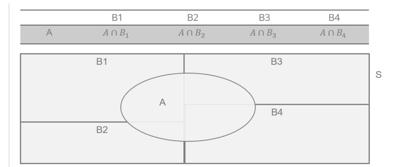
Marginal probability
The marginal probability, \(P(A)\), could be easily computed through the law of total probability. According to the law of total probability, if the events B1, B2, B3, …, Bk are mutually exclusive and collectively exhaustive (partitions of a sample space), then for any event A:
\(P(Hi/Data)\) = Posterior probability of the hypothesis Hi given the Data.
\(P(Data/Hi)\) = Likelihood of the hypothesis for some fixed data or the joint conditional probability of the data given a hypothesis.
\(P(Hi)\) = The prior probability of the hypothesis.
\(P(Data)\) = The marginal probability of the data.
Probability is the backbone of modern computational methods in statistics, data analysis, machine learning, and many other fields. The probabilistic approach to solving problems is gaining more ground today.